Microphone Position Optimization
Overview
 The aim of this student project is to evaluate and optimize the positions of microphones inside of a car to accomplish the best quality of in-car communication (ICC) systems. First a Matlab function that uses the Normalized-Least-Mean-Square (NLMS) algorithm was designed to realize an adaptive filter. Later on impulse responses were measured by applying the adaptive filter. These impulse responses represent the interior of the car. We excite the system with white noise and measure the reflected echoes with the microphones.
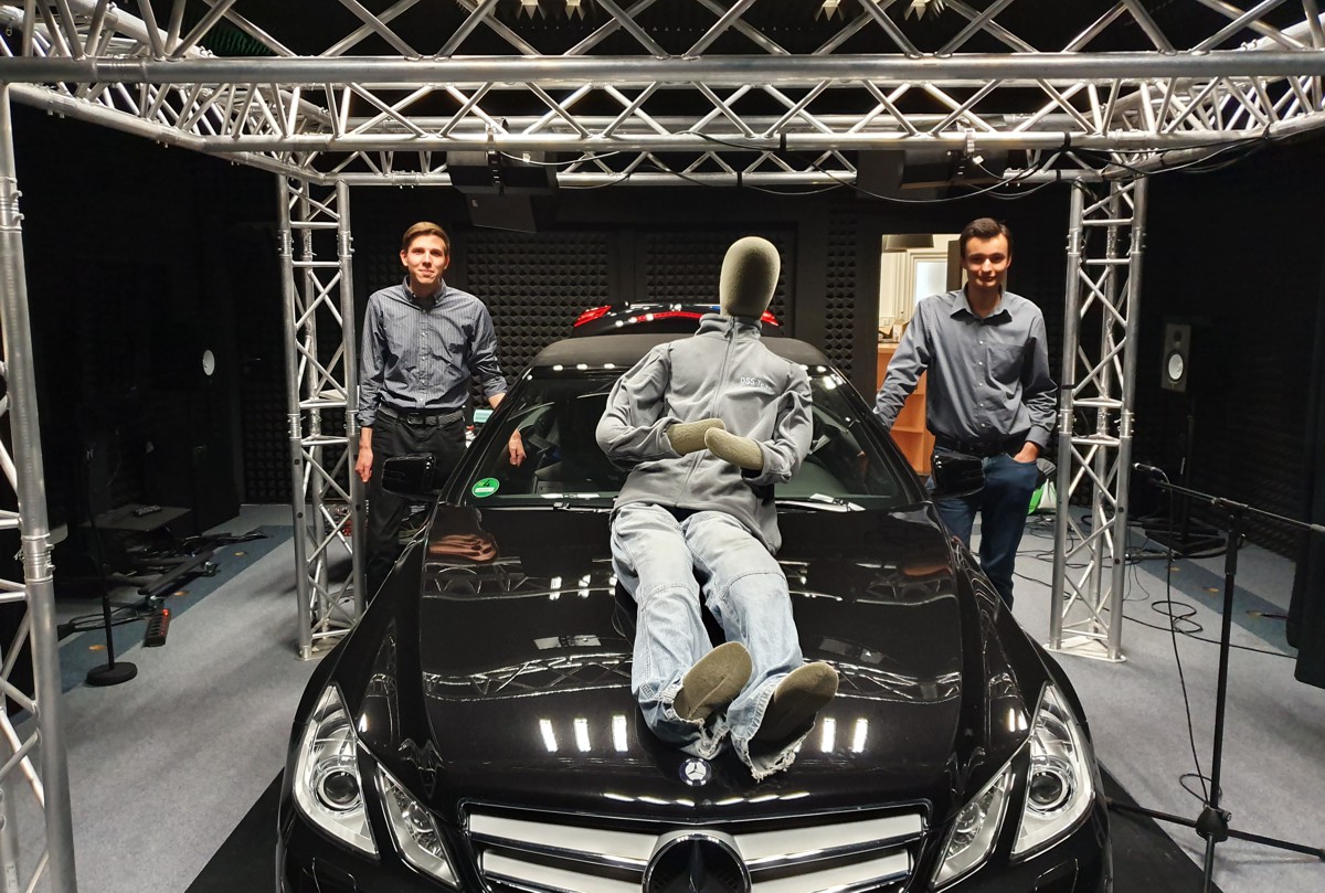
Afterwards it was time to get into the car: microphones were placed in different positions in the car. The speakers emit white noise and the microphones record the incoming signal. The given interior of the car results in different delays and different dampings because of many ways of reflection. For each position the measurement procedure was repeated to see time-variations that might result from temperature changes and other influences.
Participating Students
- Leon Neidhardt
- Dennis Zdetski
Supervisors
- Marco Gimm
- Tobias Hübschen
- Gerhard Schmidt
Implementation in Matlab
Because of the complexity of this task we couldn't just write a Matlab script to fulfill it. Instead we designed and programmed an entire interactive Matlab-Application whose main page is seen below. Expressed in numbers: It consists 3141 lines of code.
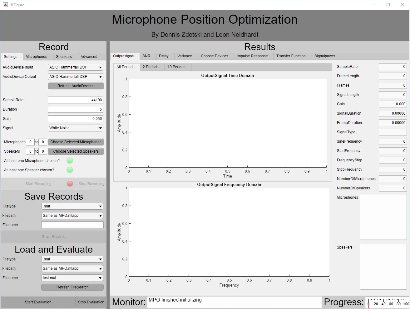
As you can see the GUI can be divided into 5 different panels: The record panel, the save-records panel, load and evaluate, the most important one: the results panel and finally the state monitor with the progress gauge.
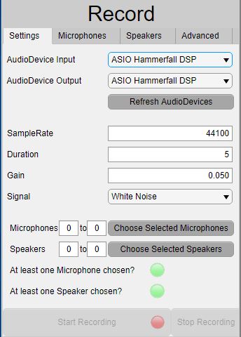 The record panel is further divided into 4 category groups that will be explained one by one.
The available audio devices and drivers are automatically imported which means that you can use the program on any computer. If any hardware changes or an audio device is added you can refresh the given devices without having to restart the program.
The signal which will be emitted by the speakers can be configured. Currently there are 3 types available: white noise, sine wave, chirp. This list can easily be extended. For each signal you can set the sample rate, the duration for how long it should be played and the gain which sets the volume.
In this menu it is also possible to choose the microphones and speakers in a form of from-to. Only if at least one microphone and one speakers is chosen both of the green lamps light up and the recording can begin. In this case the "Start Recording" button is enabled and can be pressed by the user to activate the playback and simultaneously the recording. This way many devices can be included into the measuring process without much effort.
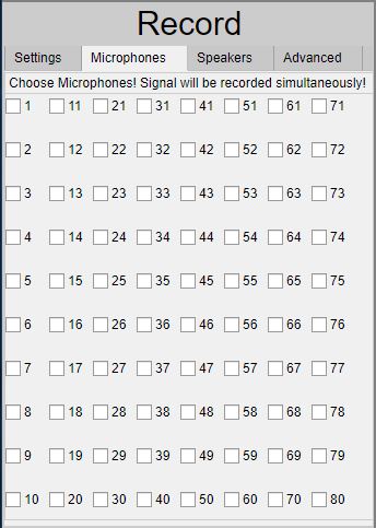 In the next menu all available recording devices are displayed. The speakers you chose in the menu before are ticked and can be set in further detail. For example if only every second speaker is plugged in. The special fact about this menu is that only the devices from the current "AudioDevice Input" are available to choose. All the others are disabled. This way you can always be sure that you only use microphones which really exist and can be used for measurement. The same page also exists for the speakers and works the same.
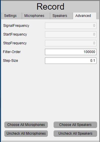 In the advanced settings you have different options for different signals. Only the ones which are available for your current choice are enabled. For the sine you can only choose one frequency while for the chirp there is a start and stop frequency to set.
In the advanced settings you have different options for different signals. Only the ones which are available for your current choice are enabled. For the sine you can only choose one frequency while for the chirp there is a start and stop frequency to set.
Additionally, there are already two settings for the evaluation: you can adapt the filter order as well as the step size of the NMLS algorithm which was mentioned in the introduction. At last there are buttons to quickly check or uncheck all microphones/speakers.
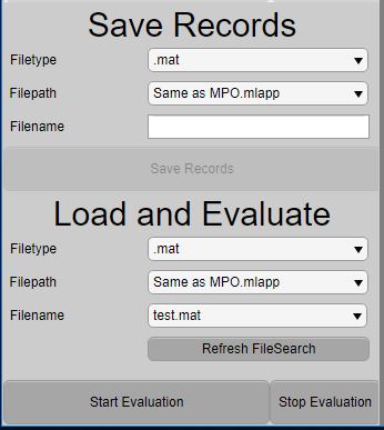 After the recording has finished you can choose the type of file and the path in which the data should be saved. This saves the raw data - no evaluation done yet. This way it can be done later due to its partly very long duration which depends on the number of speakers and microphones but especially on the filter order. The saved file can be loaded and evaluated and is automatically saved with the suffix "_evaluated".
The main assignment of the evaluation is to calculate the impulse response of the measured system. This is done with the NMLS (Normalized Least-Mean-Squares) algorithm. While processing the monitor shows the current state of evaluation and the process gauge shows the progress as a percentage. If an already evaluated file is loaded it will be directly shown in the results screen.
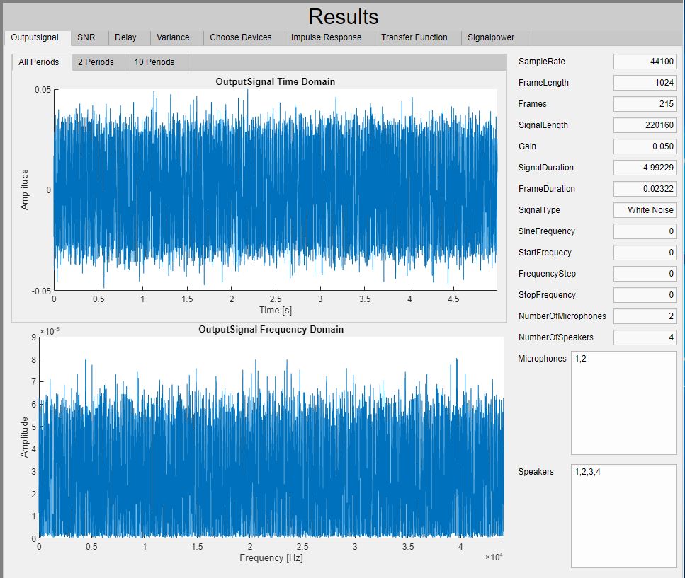
In the main panel the results can be seen after the evaluation. The first page shows the emitted output signal. You can choose between 2, 10 and all periods to show. These settings can be especially interesting for sine waves or chirps. On the right every important parameter is shown which was set before the measurement.
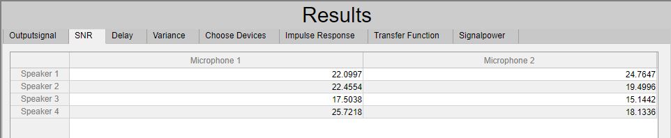
The next three figures show information relevant for every speaker-microphone combination. The first one is for the SNR. The result of the quotient of emitted signal power and received noise power which is recorded between every measurement.
The SNR tells about the quality of the signal. The higher it is the less the noise disturbed the measurement. Therefore, a good spots for microphones and speakers should have a high SNR to ensure a clear signal transmission.
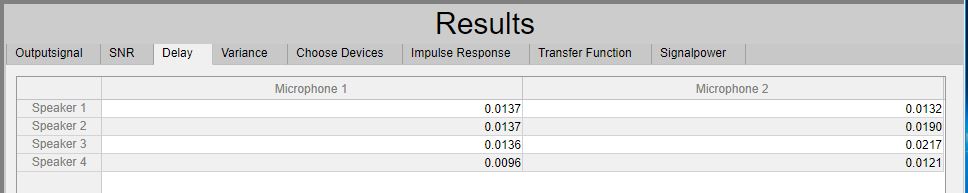
The delay screen shows the time the signal took while travelling through space. The value results from a cross-correlation between the emitted and the received signal. The number of samples the maximum is shifted leads to the delay-time. Additionally the inner-system delay is subtracted with the help of a short-circuit measurement which is made in the beginning.
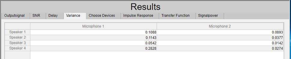
The variance shows the mathematical variance of the incoming signal in the frequency domain representing the dynamic range of each microphone-speaker combination.
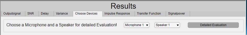
The further evaluation is displayed for every microphone-speaker combination in detail. It can be chosen in this menu.
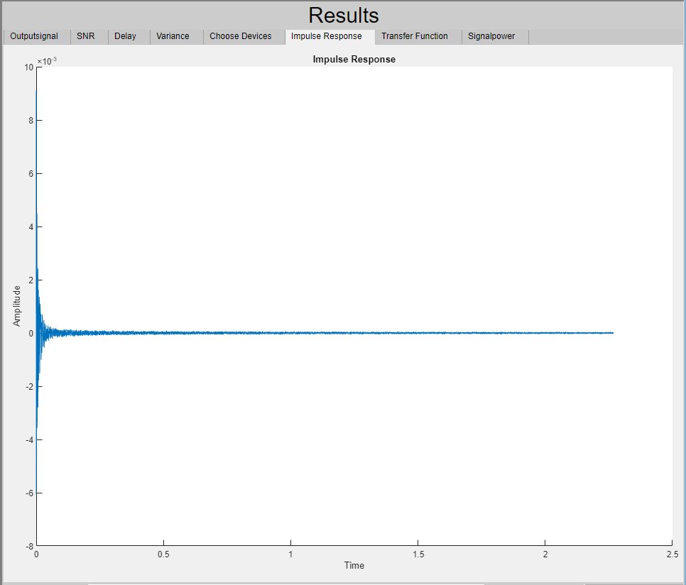
The most important part of the evaluation is the impulse response. An impulse response can as well as the transfer function represent any abstract system. It characterizes the input-output behavior of a system. The output signal can be computed by convolving the input signal with the impulse response. A single infinite small impulse at the time t=0 followed by zeros would result in a system without any delay or damping. So basically the input signal would be equal to the output signal. The more the main peak is shifted to the right the higher is the delay and the lower the peak is the higher is the damping. But in a real physical system there is not just one peak but it's followed by oscillations whose amplitudes become lower the more time passes. These oscillations represent echoes of the sound reflected by e.g. walls and are also recorded by the microphones but with a higher delay than the signal which went through the main path.
![]()
The transfer function contains the same amount of information but from another view. If the input signal is transformed into the frequency domain you can simply compute the output signal by multiplying it with the transfer function and transforming it back into the time domain. The transfer function itself is also calculated by transforming the impulse response into the frequency domain. As it's shown above the transfer function is symmetrical around half the sample rate. It is valid for all real systems.
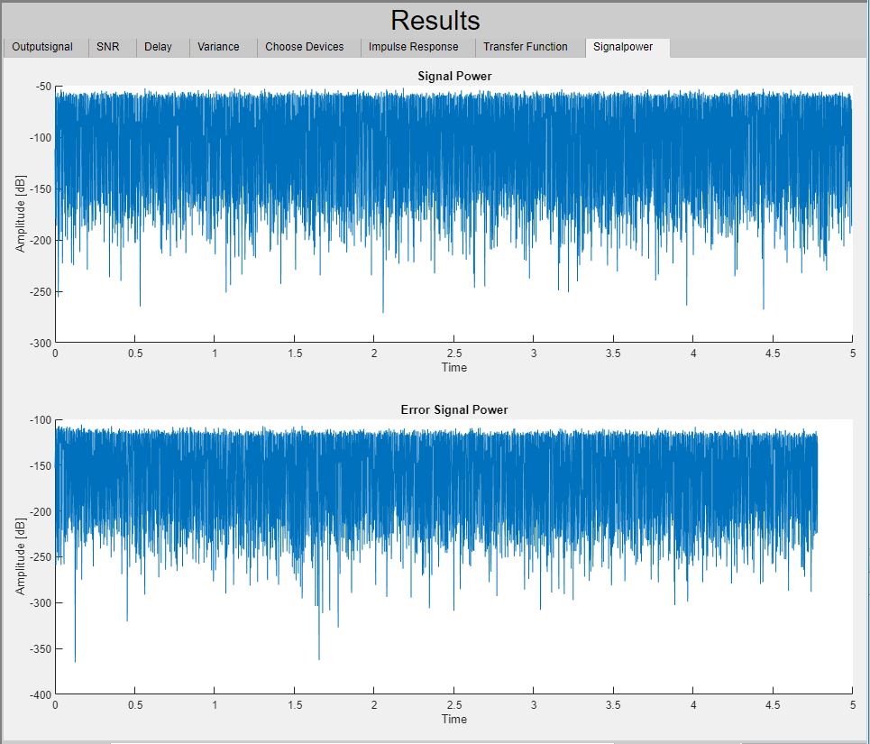
In the last two graphs you can see the signal power and the power of the error signal which is used in the calculation iterations of the NLMS algorithm. Both are calculated by squaring their amplitudes. They are about 40 - 60 dB apart from each other which is a pretty good result for the NLMS algorithm.
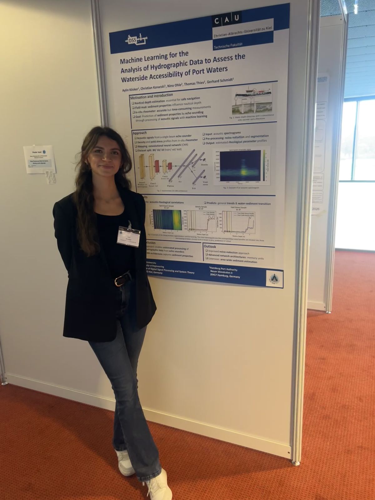 In March 2026, the DSS Chair attended the annual DAGA conference in Dresden. Thanks to the support of the GaS-Club, the student Aylin Kösker was given the opportunity to accompany the chair and participate in the conference from March 23rd to March 26th. As part of the daily poster sessions, she presented the results of her bachelor’s thesis “Machine Learning for the Analysis of Hydrographic Data to Assess the Waterside Accessibility of Port Waters” in the field of Underwater Acoustics. The thesis forms an important basis for an ongoing university research project on the acoustic analysis of sediment properties in harbor areas. The poster session enabled valuable discussions with researchers and conference participants from related research fields.