Recursive Computation of Signal Vector Norms
written by Gerhard Schmidt, Tim Owe Wisch, and Katharina Rebbe
Problem
In several signal processing applications signal vectors that contain the last \(N\) sample are utilized. Those vectors are usually defined as
\begin{equation} {\bf x}(n) \,\,=\,\, \Big[ x(n),\,x(n-1),\,x(n-2),\, ...,\,x(n-N+1)\Big]^{\textrm{T}}. \label{eq_red_rec_comp_vec_norms_00} \end{equation}
Furthermore, some applications require to compute the squared norm of such vectors. A direct computation according to
\begin{equation} \big\| {\bf x}(n)\big\|^2 \,\,=\,\, \sum\limits_{i=0}^{N-1}x^2(n-i) \label{eq_red_rec_comp_vec_norms_01} \end{equation}
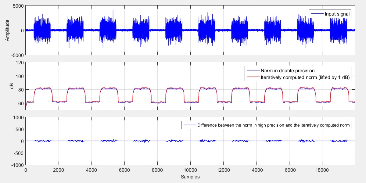
is numerically quite robust, but requires also \(N\) multiplications and \(N-1\) additions every sample. In order to show the numerical robustness, we generated a signal that contains white Gaussian noise. Every 1000 samples we varied the power by 20 dB (up and down in an alternating fashing). From that signal we extracted signal vectors of length \(N=128\) and computed the squared norm accordign to Eq. \(( \ref{eq_red_rec_comp_vec_norms_01} )\) in floating point precision, once with 64 bits and once with 32 bits and depict the results in a logarithmic fashion in Fig. 1. Additionally, the difference between the two versions is shown in the lowest diagram.
 |
||
| Fig. 1: Input signal and iterative norm computations. | ||
Recursive Computation
|
Remark: The following ideas (and the solutions) can also be used for other recursive computations such as mean estimations \(y(n) = \frac{1}{N}\sum\limits_{i=0}^{N-1}x(n-i)\). |
If the norm of the signal vector has to be computed every sample, often recursive computations are favoured since this lead to a significant recution of computational complexity - especially for signal vectors with a large amount of elements [HS 2004]. The recurive variant starts with an initialization. Is is assumed that the signal vector contains zeros at time index \(n=0\) and thus also the squared norm is initialized with zero:
\begin{eqnarray} {\bf x}(0) \,\,&=&\,\, \big[ 0,\,0,\,0,\, ...,\,0\big]^{\textrm{T}}, \\[2mm] \big\| {\bf x}(0)\big\|^2 \,\,&=&\,\, 0. \label{eq_red_rec_comp_vec_norms_02} \end{eqnarray}
Since with every sample only one new sample value is added to the signal vector and one sample value (the oldest) is leaving the vector, the norm can be computed recursively according to
\begin{equation} \big\| {\bf x}(n)\big\|^2 \,\,=\,\, \big\| {\bf x}(n-1)\big\|^2 + x^2(n) - x^2(n-N).\label{eq_red_rec_comp_vec_norms_03} \end{equation}
Using this "trick" only two multiplications and two additions are required to update the norm. However, from a numerical point-of-view, this computation is not as robust as the direct approach according to Eq. \(( \ref{eq_red_rec_comp_vec_norms_01} )\).
 |
||
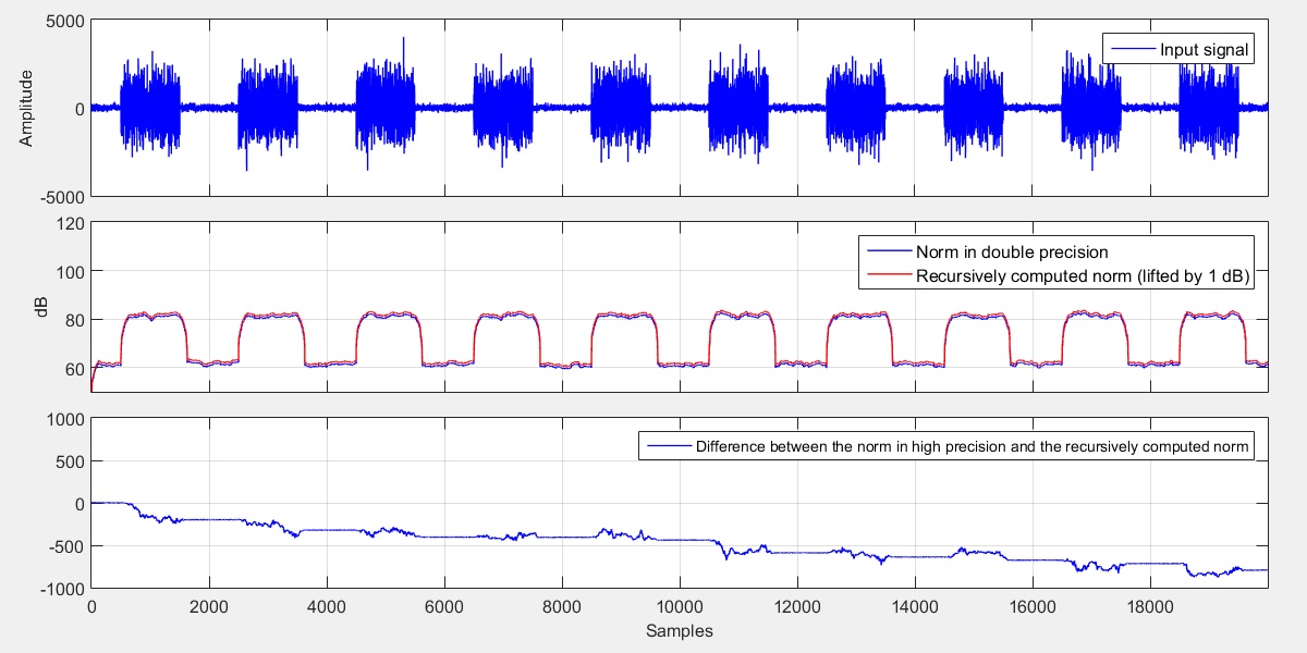
| Fig. 2: Input signal and recursive as well as iterative norm computations. | ||
The problem with the recursive computation according to Eq. \(( \ref{eq_red_rec_comp_vec_norms_03} )\) is that a squared signal value \(x^2(n)\) is used twice in the update rule:
- once when it enters the signal vector and
- once when it leaves the vector.
If the computation is done in floating-point arithmetic first the mantissa of the values that should be added or subtracted are adjusted (shifted) such that the exponents of both values are equal. This can be interpreted as some sort of quantization. If the norm value has changed between the "entering" and the "leaving" event, a small error occurs. Unfortunately, this error is biased and thus error accumulation appears.
Usually, this is not critical, because the error is really small, but if the signal has large power variations and the recursion is performed several thousand times, the small error might become rather large.
Due to that problem the norm might get negative, which leads - in some cases - to severe probelms. E.g. several gradient based optimizations perform a division by the norm of the excitation vector. If the norm gets negative it means that the direction of the gradient is switched and divergence might be the result. This could be avoided by limiting the result of the recursive computation by the value 0:
\begin{equation} \big\| {\bf x}(n)\big\|^2 \,\,=\,\, \max\Big\{0,\,\big\| {\bf x}(n-1)\big\|^2 + x^2(n) - x^2(n-N)\Big\}. \label{eq_red_rec_comp_vec_norms_04} \end{equation}
This improves robustness, but does not help against error accumulation as depicted in Fig. 2.
Mixed Recursive/Iterative Computation
A solution to this error accumulation problem is the extent the recursive computation according to Eq. \(( \ref{eq_red_rec_comp_vec_norms_04} )\) by an iterative approach that "refreshes" the recursive update from time to time. This can be realized by adding in a separate variable \(N_{\textrm{rec}}(n)\) all squared input samples:
\begin{equation} N_{\textrm{rec}}(n) \,\,=\,\, \left\{ \begin{array}{ll} x^2(n), & \textrm{if}\,\mod(n,N)\,\equiv\, 0, \\[2mm] N_{\textrm{rec}}(n-1) + x^2(n), & \textrm{else}. \end{array}\right. \label{eq_red_rec_comp_vec_norms_05} \end{equation}
If \(N\) samples are added this variable is replacing to the recursively computed norm and the original sum \(N_{\textrm{rec}}(n)\) is reinitialized with 0:
\begin{equation} \big\| {\bf x}(n)\big\|^2 \,\,=\,\, \left\{ \begin{array}{ll} N_{\textrm{rec}}(n), & \textrm{if}\,\mod(n,N)\,\equiv\, N-1, \\[2mm] \max\Big\{0,\,\big\| {\bf x}(n-1)\big\|^2 + x^2(n) - x^2(n-N)\Big\},& \textrm{else}. \end{array}\right. \label{eq_red_rec_comp_vec_norms_06} \end{equation}
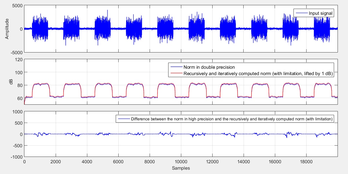
The additional mechanism adds only a few additions, but helps a lot against error accumulation as indicated in the last example of this section depicted in Fig. 3. Thus, if you face problems with norms of signal vectors you might think about using this mixed method.
 |
||
| Fig. 3: Input signal and mixed recursive/iterative as well as purely iterative norm computations. | ||
References
| [HS 2004] | E. Hänsler, G. Schmidt: Acoustic Echo and Noise Control, Wiley, 2004. |
Code Example
As usual you can find below some matlab code that shows examples on the inidvidual methods of norm computations as well as the corresponding analyses.
{slider title="Different methods of computing vector norms" class="grey" open="false"}
%**************************************************************************
% Parameters
%**************************************************************************
N            =   128;
Sig_duration = 10000;

%**************************************************************************
% Generate input signal
%**************************************************************************

% Generate white Gaussian noise
sig = single(randn(Sig_duration,1));

% Boost every second 1000 signal values by 60 dB
for k = 1001:2000:Sig_duration;
    sig(k-1000:k) = sig(k-1000:k) * 1000;
end;

%**************************************************************************
% Compute norms
%**************************************************************************
x_vec               = single(zeros(N,1));
Norm_rec_curr       = single(0);
Norm_rec_curr_lim   = single(0);
N_rec               = single(0);
C_rec               = single(0);
Norm_mixed_curr     = single(0);
N_rec_lim           = single(0);
C_rec_lim           = single(0);
Norm_mixed_lim_curr = single(0);

Norm_double_prec    = zeros(Sig_duration,1);
Norm_iterative      = single(zeros(Sig_duration,1));
Norm_recursive      = single(zeros(Sig_duration,1));
Norm_recursive_lim  = single(zeros(Sig_duration,1));
Norm_mixed          = single(zeros(Sig_duration,1));
Norm_mixed_lim      = single(zeros(Sig_duration,1));

for k = 1:Sig_duration

    %**********************************************************************
    % Update signal vector (not very efficient, but o.k. for here
    %**********************************************************************
    x_new      = sig(k);
    x_old      = x_vec(N);
    x_vec(2:N) = x_vec(1:N-1);
    x_vec(1)   = x_new;

    %**********************************************************************
    % Norm in double precicion
    %**********************************************************************
    Norm_double_prec(k) = double(x_vec)' * double(x_vec);

    %**********************************************************************
    % Iterative norm (of course, there exixt optimized Matlab functions
    % for this purpose, but that's another "story")
    %**********************************************************************
    for n = 1:N
        Norm_iterative(k) = Norm_iterative(k) + x_vec(n)*x_vec(n);
    end;

    %**********************************************************************
    % Recursive norm computation
    %**********************************************************************
    Norm_rec_curr     = Norm_rec_curr + x_new^2 - x_old^2;
    Norm_recursive(k) = Norm_rec_curr;

    %**********************************************************************
    % Recursive norm computation
    %**********************************************************************
    Norm_rec_curr_lim     = Norm_rec_curr_lim + x_new^2 - x_old^2;
    Norm_rec_curr_lim     = max(0, Norm_rec_curr_lim);
    Norm_recursive_lim(k) = Norm_rec_curr_lim;

    %**********************************************************************
    % Mixed compuation of the norm
    %**********************************************************************
    Norm_mixed_curr = Norm_mixed_curr + x_new^2 - x_old^2;

    C_rec = C_rec + 1;
    if (C_rec == N)
        C_rec = 0;
    end;

    if (C_rec == 0)
        N_rec = 0;
    end;
    N_rec = N_rec + + x_new^2;

    if (C_rec == N-1)
        Norm_mixed_curr = N_rec;
    end;

    Norm_mixed(k) = Norm_mixed_curr;

    %**********************************************************************
    % Mixed compuation of the norm with limiation
    %**********************************************************************
    Norm_mixed_lim_curr = Norm_mixed_lim_curr + x_new^2 - x_old^2;
    Norm_mixed_lim_curr = max(0,Norm_mixed_lim_curr);

    C_rec_lim = C_rec_lim + 1;
    if (C_rec_lim == N)
        C_rec_lim = 0;
    end;

    if (C_rec_lim == 0)
        N_rec_lim = 0;
    end;
    N_rec_lim = N_rec_lim + + x_new^2;

    if (C_rec_lim == N-1)
        Norm_mixed_lim_curr = N_rec_lim;
    end;

    Norm_mixed_lim(k) = Norm_mixed_lim_curr;

end;

%**************************************************************************
% Show results
%**************************************************************************
fig = figure(1);
set(fig,'Units','Normalized');
set(fig,'Position',[0.1 0.1 0.8 0.8]);

t = 0:Sig_duration-1;

subplot('Position',[0.07 0.8 0.9 0.17]);
plot(t,10*log10(Norm_double_prec),'b', ...
     t,10*log10(max(0.01, Norm_iterative))+1,'r');
grid on
set(gca,'XTickLabel','');
ylabel('dB')
legend('Norm in double precision', ...
       'Iteratively computed norm (lifted by 1 dB)');
axis([0 Sig_duration-1 0 120]);

subplot('Position',[0.07 0.62 0.9 0.17]);
plot(t,10*log10(Norm_double_prec),'b', ...
     t,10*log10(max(0.01, Norm_recursive))+1,'r');
grid on
set(gca,'XTickLabel','');
ylabel('dB')
legend('Norm in double precision', ...
       'Recursively computed computed norm (lifted by 1 dB)');
axis([0 Sig_duration-1 0 120]);

subplot('Position',[0.07 0.44 0.9 0.17]);
plot(t,10*log10(Norm_double_prec),'b', ...
     t,10*log10(max(0.01, Norm_recursive_lim))+1,'r');
grid on
set(gca,'XTickLabel','');
ylabel('dB')
legend('Norm in double precision', ...
       'Recursively computed computed norm with limitation (lifted by 1 dB)');
axis([0 Sig_duration-1 0 120]);

subplot('Position',[0.07 0.26 0.9 0.17]);
plot(t,10*log10(Norm_double_prec),'b', ...
     t,10*log10(max(0.01, Norm_mixed))+1,'r');
grid on
set(gca,'XTickLabel','');
ylabel('dB')
legend('Norm in double precision', ...
       'Mixed recursively/iteratively computed norm (lifted by 1 dB)');
axis([0 Sig_duration-1 0 120]);

subplot('Position',[0.07 0.08 0.9 0.17]);
plot(t,10*log10(Norm_double_prec),'b', ...
     t,10*log10(max(0.01, Norm_mixed_lim))+1,'r');
grid on
xlabel('Samples');
ylabel('dB')
legend('Norm in double precision', ...
       'Mixed recursively/iteratively computed norm with limitation (lifted by 1 dB)');
axis([0 Sig_duration-1 0 120]);
{/sliders}


