Removal of Signal Trends

written by Christin Bald, Julia Kreisel, and Gerhard Schmidt

Problem

In several applications signals are recorded that contain an offset. Sometimes the offset carries Information - in these cases this signal component should not be removed. However, in a variety of applications one is interested mainly in the temporal variations of the signal (and not in the offset). In these cases a simple (meaning computationally efficient) and robust offset or so-called trend removal can be applied. This allows follow-up signal processing to be a bit simpler, e.g. thresholds do not have to be adjusted to the offset.

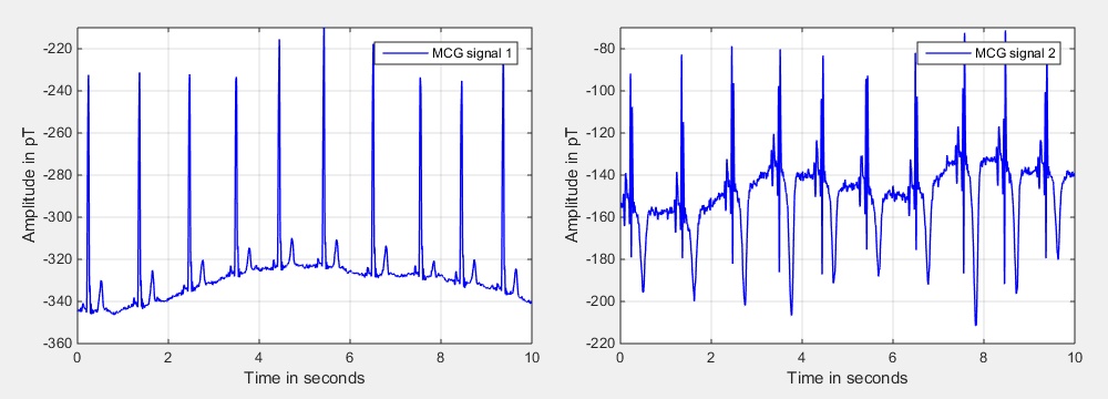
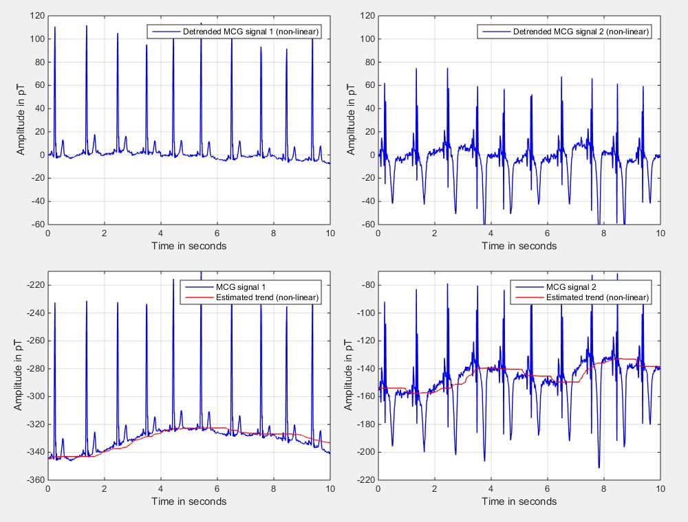
Examples for such signals are ECG or MCG signals, where ECG abbreviates electrocardiogram and MCG its magnetic counterpart, magnetocardiogram. Since the authors work with the analysis of both we will use MCG signals as an example. Fig. 1 shows two signals that were recorded at the same time but at different positions.

	Fig. 1: MCG (magnetocardiogram) input signals.

MCG signals show the same cardiac cycle as known from ECG signals. One heart cycle consists of a P wave, a QRS complex, and a T wave [P 2011]. The first wave is the P wave in which the atria contraction is described. The QRS complex is the combination of the Q, R and S wave showing the beginning of the contraction of the ventricle. The start of the T wave describes the beginning of the relaxation. The offset means an almost constant shifting from zero.

A Simple Method to Remove a Signal Offset

A very simple method to remove the trend in a signal is to know the trend a priori and to subtract this value. If the application allows for a so-called pre-measurement, it is rather simple to obtain an estimate for the mean of the signal (with or without the desired signal component). Assuming that we have this measure, we can obtain a simple trend estimate by just using the a priori knowledge:

\begin{eqnarray} x_\textrm{trend,simple}(n) &=& x_\textrm{a prioi}. \label{Eq:TrendRemoval_Offset_Removal_01} \end{eqnarray}

The trend compensated signal can be obtained by subtracting the estimated trend from the measured signal:

\begin{eqnarray} x_\textrm{comp,simple}(n) &=& x(n) - x_\textrm{trend,simple}(n). \label{Eq:TrendRemoval_Offset_Removal_02} \end{eqnarray}

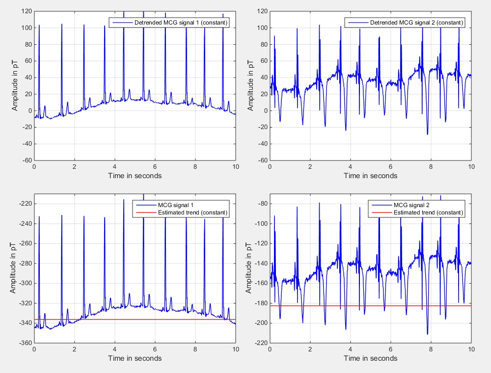
To obtain a good estimate for $x_\textrm{a priori}$ we have averaged the two input signals that are depicted in Fig. 1 for the entire length of both signals individually. The resulting values are then used as a priori knowledge and are subtracted from the input signals according to Eq. $(\ref{Eq:TrendRemoval_Offset_Removal_02})$. Fig. 2 shows the resulting detrended signals (in the upper diagrams) as well as the estimated trends (red color) and the input signals (blue color) in the lower diagrams. Please note that only the first 10 seconds of the signals are depicted. The second signal gets a much smaller offset during the period of 10 to 30 seconds (compared to the first 10 seconds), leading to the depicted average that looks a bit too small at first glance.

	Fig. 2: Input signals, estimated trends, and trend compensated signals using the method of constant subtraction.

Removal of Signal Trends by Highpass Filtering

A second method for trend removal is to estimate the mean of the signal by means of averaging the signal over the last $N_\textrm{hp}$ samples:

\begin{eqnarray} x_\textrm{trend,hp}(n) &=& \frac{1}{N_\textrm{hp}} \sum\limits_{i=0}^{N_\textrm{hp}-1} x(n-i). \label{Eq:TrendRemoval_Highpass_01} \end{eqnarray}

The estimated mean value $x_\textrm{trend,hp}(n)$ is subtracted from the input signal

\begin{eqnarray} x_\textrm{comp,hp}(n) &=& x(n) - x_\textrm{trend,hp}(n), \label{Eq:TrendRemoval_Highpass_02} \end{eqnarray}

resulting in the desired trend removal. While Eq.$(\ref{Eq:TrendRemoval_Highpass_01})$ describes a lowpass filter, the subtraction in Eq. $(\ref{Eq:TrendRemoval_Highpass_02})$ results in a highpass filter, which gives this section also its name. Both filters are related (in the frequency domain) as:

\begin{eqnarray} H_\textrm{hp}\big(e^{-j\Omega}\big) &=& 1 - H_\textrm{lp}\big(e^{-j\Omega}\big). \label{Eq:TrendRemoval_Highpass_03} \end{eqnarray}

The frequency response of the lowpass filter can be obtained by first having a closer look on Eq. $(\ref{Eq:TrendRemoval_Highpass_01})$ in the time domain. The equation can be interpreted as a convolution of the input signal with the lowpass impulse response $h_{\textrm{lp,} n}$:

\begin{eqnarray} x_\textrm{trend,hp}(n) &=& \sum\limits_{i=\infty}^{\infty} h_\textrm{lp,$i$}\,x(n-i). \label{Eq:TrendRemoval_Highpass_04} \end{eqnarray}

Comparing Eqs. $(\ref{Eq:TrendRemoval_Highpass_01})$ and $(\ref{Eq:TrendRemoval_Highpass_04})$ leads to the FIR (finite impulse response, [M 2001, PM 1996, T 1983]) system

\begin{eqnarray} h_{\textrm{lp,} i} &=& \left\{ \begin{array}{ll} \displaystyle{\frac{1}{N_\textrm{hp}}}, & \textrm{if}\,\,0 \le i < N_\textrm{hp}, \\[3mm] 0, & \textrm{else}. \end{array} \right. \label{Eq:TrendRemoval_Highpass_05} \end{eqnarray}

Taking also the subtraction of Eq. $(\ref{Eq:TrendRemoval_Highpass_02})$, which actually detrends the signal, into account leads to the impulse response of the high pass filter (again an FIR filter):

\begin{eqnarray} h_{\textrm{hp,}i} &=& \left\{ \begin{array}{ll} \displaystyle{1 - \frac{1}{N_\textrm{hp}}}, & \textrm{if}\,\,i = 0, \\[3mm] \displaystyle{-\frac{1}{N_\textrm{hp}}}, & \textrm{if}\,\,1 \le i < N_\textrm{hp}, \\[3mm] 0, & \textrm{else}. \end{array} \right. \label{Eq:TrendRemoval_Highpass_06} \end{eqnarray}

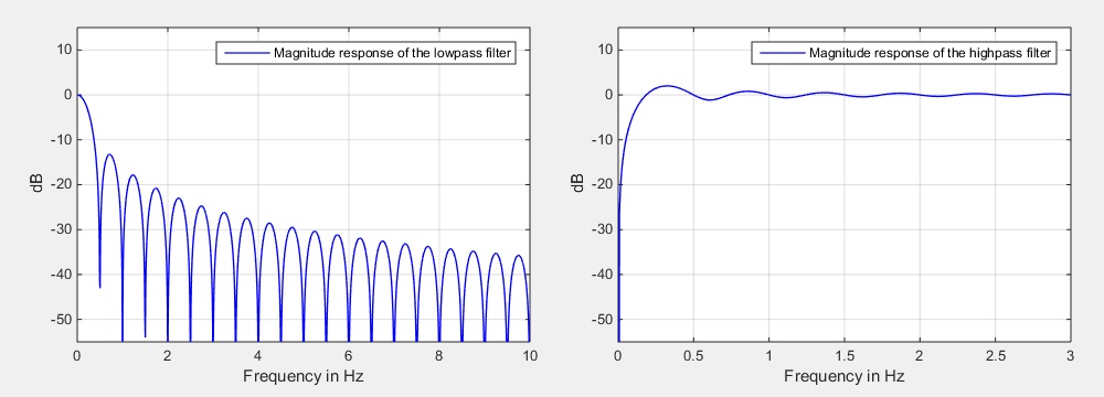
In Fig. 2 the magnitude responses of resulting lowpass (left side) and highpass filter (right side) are depicted. For a sample rate of $f_\textrm{s} = 1000$ Hz a filter order $N_\textrm{hp} = 2000$ was chosen, leading to an average based on the last two seconds of the signal.

	Fig. 3: Magnitude responses of the lowpass and highpass filter for a filter order of $N_\textrm{hp} = 2000$ and a sample rate of $f_\textrm{s} = 1000$ Hz.

The computation of the lowpass part of the trend removal is rather costly, since usually a few hundred or even thousand (as in our example) signals have to be added. Of course, one can speed up the process by performing the entire operation in the spectral domain using fast Fourier transforms. However, this would introduce delay due to the necessary framing. Another way that is able to save an even larger amount of complexity is to exploit the special choice of the filter coefficients (they are all the same) and transform the FIR filter into an IIR structure. This can be achieved by recursively computing the estimated trend according to

\begin{eqnarray} x_\textrm{trend,hp}(n) &=& x_\textrm{trend,hp}(n-1) + \frac{1}{N_\textrm{hp}} \, \Big[ x(n) - x(n-N_\textrm{hp}) \Big]. \label{Eq:TrendRemoval_Highpass_07} \end{eqnarray}

This requires only two additions and one multiplication per sample. Please note that the division by $N_\textrm{hp}$ can be computed during initialization and the inverse value can be stored. This transforms the division into a multiplication (at least for the main operation of the filter). In terms of memory nothing has changed with this trick - still $N_\textrm{hp}$ samples have to be stored in a so-called ringbuffer.

Transforming specific FIR filter structures into equivalent IIR counterparts is not new. However, only a few authors mention the numerical problems that appear with this kind of processing.

When computing Eq. $(\ref{Eq:TrendRemoval_Highpass_07})$ on a processor with floating point precision, the mantissae of all terms that should be added are shifted until the exponents are all the same. When a sample is entering the memory this shifting operation is not necessarily the same as during the leaving event. As a consequence biased error accumulation appears. If the signal is rather short this is not really an issue. However, if a few thousand samples have to be processed this might lead to numerical problems.

A solution to this problem is rather simple. The recursive processing should be updated from time to time by an iteratively computed estimation. This could be achieved with a small extension to Eq. $(\ref{Eq:TrendRemoval_Highpass_07})$:

\begin{eqnarray} x_\textrm{trend,hp}(n) &=& \left\{ \begin{array}{ll} \displaystyle{\frac{x_\textrm{trend,reset}(n)}{N_\textrm{hp}}}, & \textrm{if}\,\mod(n,N_\textrm{hp}) \equiv N_\textrm{hp}-1,\\[2mm] x_\textrm{trend,hp}(n-1) + \displaystyle{\frac{1}{N_\textrm{hp}}} \Big[ x(n) - x(n-N_\textrm{hp}) \Big], & \textrm{else}. \end{array} \right. \label{Eq:TrendRemoval_Highpass_08} \end{eqnarray}

The so-called reset value can be computed according to

\begin{eqnarray} x_\textrm{trend,reset}(n) &=& \left\{ \begin{array}{ll} x(n), & \textrm{if}\,\mod(n,N_\textrm{hp}) \equiv 0, \\[2mm] x_\textrm{trend,reset}(n-1) + x(n), & \textrm{else}. \end{array} \right. \label{Eq:TrendRemoval_Highpass_9} \end{eqnarray}

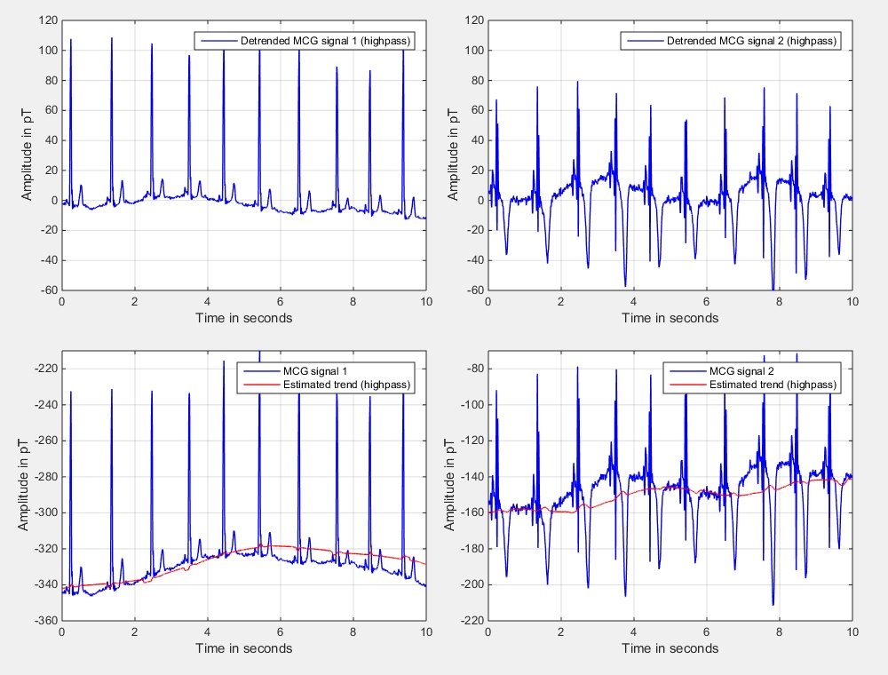
To show the results of this second method, the simulation of Fig. 2 has been repeated, but now with the highpass method. Fig. 4 shows in the upper diagrams the detrended results as well as the input signals (blue color) and the estimated trends (red color) in the lower diagrams.

	Fig. 4: Input signals, estimated trends, and trend compensated signals using highpass filtering.

A Non-linear and Time-variant Approach

As a last method we would like to introduce a non-linear, time-variant method. The method is nearly as simple as the highpass filter, but is usually a bit better, especially if the short-term mean of the signal is not zero. In addition a significant reduction of the required memory (compared to the highpass filter approach) is possible.

As a first step we define the global memory of the signal as $N_\textrm{global}$ samples. In the following we will base our analyses on input signals up to that delay. Please note that it is not required to store the input signal for that amount of samples. As a second step we split the global memory into frames and define the framesize $N_\textrm{frame}$ for our method. For the MCG example we could use about 1 second of global memory and a frame duration of about 100 ms. Since the data was sampled at $f_\textrm{s} = 1$ kHz, we get

\begin{eqnarray} N_\textrm{global} &=& 1000, \label{Ed:TrendRemoval_Nonlinear_01a} \\[2mm] N_\textrm{frame} &=& 100. \label{Ed:TrendRemoval_Nonlinear_01b} \end{eqnarray}

Furthermore, we assume that $N_\textrm{global}$ is an integer multiple of $N_\textrm{frame}$

\begin{eqnarray} N_\textrm{global} &=& K_\textrm{frame}\,N_\textrm{frame}, \label{Ed:TrendRemoval_Nonlinear_02} \end{eqnarray}

which is true in the example above ($K_\textrm{frame} = 10$). As a next step we compute in an iterative manner the mean for each frame according to

\begin{eqnarray} x_\textrm{curr. mean}(n) = \left\{ \begin{array}{ll} \displaystyle{\frac{x(n)}{N_\textrm{frame}}}, & \textrm{if}\,\,\textrm{mod}\big(n,N_\textrm{frame}\big) \equiv 0, \\[2mm] x_\textrm{curr. mean}(n-1) + \displaystyle{\frac{x(n)}{N_\textrm{frame}}}, & \textrm{else.} \end{array} \right. \label{Ed:TrendRemoval_Nonlinear_03} \end{eqnarray}

Please note that $x_\textrm{curr. mean}(n)$ only results in the correct mean if the condition

\begin{eqnarray} n &=& \lambda\,N_\textrm{frame}-1, \label{Ed:TrendRemoval_Nonlinear_04} \end{eqnarray}

is true (with $\lambda \in \mathcal{Z})$. To save computational complexity the division by $N_\textrm{frame}$ can also be avoided for the sample-by-sample iteration - it should be performed only when the frame is completely filled. Beside the simple update according to Eq. $(\ref{Ed:TrendRemoval_Nonlinear_03})$ only one first-order recursive smoothing process and the subtraction of the estimated trend according to

\begin{eqnarray} x_\textrm{comp,nl}(n) &=& x(n) - x_\textrm{trend,nl}(n) \label{Ed:TrendRemoval_Nonlinear_05} \end{eqnarray}

are computed at the high sample rate. All other computations are computed only once per $N_\textrm{frame}$ samples. It will lead to a trend estimate $\tilde x_\textrm{trend,nl}(n)$ that is available only if

\begin{eqnarray} \textrm{mod}\big(n,N_\textrm{frame}\big) &\equiv& N_\textrm{frame}-1, \label{Ed:TrendRemoval_Nonlinear_06} \end{eqnarray}

which is an equivalent condition to Eq. $(\ref{Ed:TrendRemoval_Nonlinear_04})$. If we would use the (subsamples) estimated trend directly in Eq. $(\ref{Ed:TrendRemoval_Nonlinear_05})$, sudden signal jumps might appear. For that reason, first order IIR smoothing is performed to avoid such artifacts:

\begin{eqnarray} x_\textrm{trend,nl}(n) = \beta_\textrm{sm} \, x_\textrm{trend,nl}(n-1) + (1 - \beta_\textrm{sm})\, \tilde x_\textrm{trend,nl}\Big( \Big\lfloor \frac{n}{N_\textrm{frame}}\Big\rfloor \Big). \label{Ed:TrendRemoval_Nonlinear_07} \end{eqnarray}

The symbols $\lfloor ... \rfloor$ should indicate rounding down. The smoothing parameter $\beta_\textrm{sm}$ is chosen from the interval

\begin{eqnarray} 0 \ll \beta_\textrm{sm} < 1. \label{Ed:TrendRemoval_Nonlinear_08} \end{eqnarray}

Typically $\beta_\textrm{sm}$ is chosen out of the range $[0.9,\,0.9999]$ -- depending on the sample rate $f_\textrm{s}$ and on the frame size $N_\textrm{frame}$. If a frame is completely filled (according to condition $(\ref{Ed:TrendRemoval_Nonlinear_06})$ the short-term mean is added to a vector that contains the last $K_\textrm{frame}$ short-term means

\begin{eqnarray} {\bf x}_\textrm{mean}(n) &=& \left\{ \begin{array}{l} \Big[x_\textrm{curr. mean}\big(n\big),\,x_\textrm{curr. mean}\big(n-N_\textrm{frame}\big),\, ...,\,x_\textrm{curr. mean}\big(n-(K_\textrm{frame}-1)N_\textrm{frame}\big) \Big]^{\textrm{T}}, \\[2mm] \qquad \textrm{if} \,\,\textrm{mod}(n,N_\textrm{frame}) \equiv N_\textrm{frame}-1, \\[4mm] {\bf x}_\textrm{mean}(n-1), \\[2mm] \qquad \textrm{else}. \end{array} \right. \nonumber \\ \label{Ed:TrendRemoval_Nonlinear_09} \end{eqnarray}

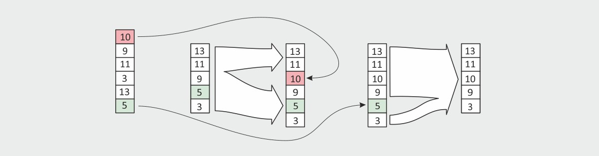
This method allows to store the supporting points of the averaged signal in a subsampled manner, meaning that only $K_\textrm{frame}$ data words (in our example 10) are required to store information of $N_\textrm{global}$ samples (in our example 1000). The basic idea to estimate the trend is now to sort the entries of the vector ${\bf x}_\textrm{mean}(n)$ and to utilize, e.g., the median of the stored short-term means. Beside the median also other quantiles could be utilized. However, the median usually should be the first choice. The vector containing the sorted mean values is denoted by

\begin{eqnarray} {\bf x}_\textrm{mean, sorted}(n) &=& \Big[ x_\textrm{mean, sorted, 0}(n),\,x_\textrm{mean, sorted, 1}(n),\,...,\,x_\textrm{mean, sorted, $K_\textrm{frame}-1$}(n) \Big]^{\textrm{T}}. \end{eqnarray}

The reason for using a sorting operation here (and not a second averaging stage) is that this allows also for a good trend estimation even if the signal might have a positive or negative bias (as it is the case in the first MCG example signal). Of course the literature is full of efficient sorting algorithms. However, since we can assume that we already have a sorted list available before a new short-term mean is computed we can use a two-stage procedure that updates the sorted list:

• As a first stage we copy the old sorted vector and the new short-term mean into an extended sorted vector. This operation can be performed with $K_\textrm{frame}+1$ operations.

• In a second stage we copy the extended vector back into the original. Beside this copying operation we check if the element to be copied is equal to the short-term mean that leaves the vector ${\bf x}_\textrm{mean}(n)$. This element is then not copied resulting in a shortening of the extended vector. For this second part again $K_\textrm{frame}+1$ operations are required.

As a consequence the entire sorting procedure (which is actually only an update of an already sorted list) required only about $2\,K_\textrm{frame}$ operations. Fig. 5 shows an overview about the two-stage sorting procedure.

	Fig. 5: Sorting of the frame means.

Every $N_\textrm{frame}$ sample the (non-smoothed) trend estimate is updated according to

\begin{eqnarray} \tilde x_\textrm{trend,nl}(n) &=& \left\{ \begin{array}{ll} x_{\textrm{mean, sorted,} K_\textrm{frame}/2}(n), & \textrm{if}\,\,\textrm{mod}(n,N_\textrm{frame}) \equiv N_\textrm{frame}-1, \\[2mm] \tilde x_\textrm{trend,nl}(n-1), & \textrm{else}. \end{array} \right. \label{Ed:TrendRemoval_Nonlinear_10} \end{eqnarray}

As in the last sections we perform the detrending operation with the two MCG input signals and show the estimated trends together with the input signals as well as the detrended signals in Fig. 6.

	Fig. 6: Input signals, estimated trends, and trend compensated signals using the non-linear and time-variant approach.

Comparison of the Three Methods

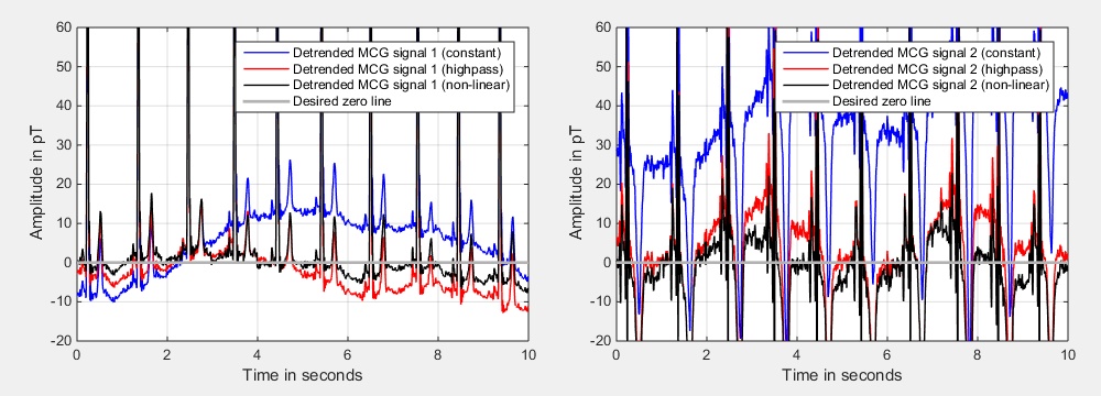
In comparison to the other two methods, the first one is the simplest one. As one can see in Fig. 7 the method removes the trend (at least partly), but the resulting signal is not really on the desired zero line. However, the required computing time is really low since only a fixed constant is subtracted. Also nearly no memory (one data word for the mean) is required. The method using the highpass approach gives a quite good result but needs the largest memory. In addition, the highpass method requires a little bit more computing time, but still only a few operations are required per sample if computed in recursive manner. The non-linear method fits nearly exactly to the zero line. Furthermore, much less memory is required (compared to the highpass method). As conclusion one can say that the non-linear method is the best for removing offsets -- at least for the examples that we tested here.

	Fig. 7: Comparison of the three methods.

References

Code Example

As usual you can find below some matlab code that shows three different methods to remove the trend of a signal.

%**************************************************************************
% Clear and close everything
%**************************************************************************
clc;
clear all;
close all;

%**************************************************************************
% Load input data
%**************************************************************************
[sig, f_s] = audioread('mcg_01.wav');

%**************************************************************************
% Detrending - Method 1: Subtraction of constant (mean)
%**************************************************************************
sig_detr_const = sig - mean(sig);

%**************************************************************************
% Detrending - Method 2: Highpass
%**************************************************************************

% Parameters **************************************************************
N_hp    = 2*f_s;

% Initializations *********************************************************
mean_start      = mean(sig);
sig_detr_hp     = zeros(size(sig));
est_mean_sig_hp = zeros(size(sig));
sig_mem         = zeros(N_hp,1) + mean_start;
ptr_sig         = 0;
mean_rec        = mean_start;
mean_iter       = 0;
k_iter          = 0;
N_hp_inv        = 1 / N_hp;

%**************************************************************************
% Main loop 
%**************************************************************************
for k = 1:length(sig)
    
    %**********************************************************************
    % Get new input signal
    %**********************************************************************
    sig_entering = sig(k);
    
    %**********************************************************************
    % Update ring buffer
    %**********************************************************************
    % Update of the pointer (modulo N_hp) *********************************
    ptr_sig = ptr_sig + 1;
    if (ptr_sig > N_hp)
        ptr_sig = 1;
    end
    
    % Store leaving signal in variable ************************************
    sig_leaving      = sig_mem(ptr_sig);
    
    % Add new input to signal memory **************************************
    sig_mem(ptr_sig) = sig_entering;
    
    %**********************************************************************
    % Update mean recursively
    %**********************************************************************
    mean_rec = mean_rec + (sig_entering - sig_leaving) * N_hp_inv;
    
    %**********************************************************************
    % Iteratively computed mean and correction of rec. mean
    %**********************************************************************
    k_iter    = k_iter + 1;
    mean_iter = mean_iter + sig_entering; 
    if (k_iter == N_hp)
        mean_rec  = mean_iter * N_hp_inv;
        mean_iter = 0;
        k_iter    = 0;
    end
    
    %**********************************************************************
    % Store estimated mean (for analysis purposes)
    %**********************************************************************
    est_mean_sig_hp(k) = mean_rec;
    
    %**********************************************************************
    % Output = input - mean
    %**********************************************************************
    sig_detr_hp(k) = sig_entering - mean_rec;    
end

%**************************************************************************
% Detrending - Method 3: New method (no name found yet)
%**************************************************************************

% Parameters **************************************************************
Cell_dur       = round(0.1 * f_s);           % Cell duration
N_mem_des      = round(1.0 * f_s);           % Total memory duration
N_cells        = round(N_mem_des/Cell_dur);  % Number of cells
mean_start     = mean(sig);
beta_sm        = 0.98; 

% Initializations *********************************************************
detr_counter              = 0;
Cell_dur_inv              = 1 / Cell_dur;   
mean_curr_cell            = 0; 
vec_cell_means            = zeros(N_cells,1)   + mean_start;
vec_cell_means_sorted     = zeros(N_cells,1)   + mean_start;
vec_cell_means_sorted_ext = zeros(N_cells+1,1) + mean_start;
pointer_vec_cell_means    = 0;
global_mean_est           = mean_start;   
sig_detr_new              = zeros(size(sig));
est_mean_sig_new          = zeros(size(sig));
global_mean_est_sm        = mean_start;

%**************************************************************************
% Main loop 
%**************************************************************************
for k = 1:length(sig)

    %**********************************************************************
    % Get new input signal
    %**********************************************************************
    sig_entering = sig(k);
    
    %**********************************************************************
    % Increment main counter
    %**********************************************************************
    detr_counter = detr_counter + 1;
    
    if (detr_counter > Cell_dur - 1)  
    
        % Reset counter ***************************************************
        detr_counter = 0;
        
        % Use current sample **********************************************
        mean_curr_cell = mean_curr_cell + sig(k);
        
        % Finalize estimation of mean of current cell *********************
        mean_curr_cell = mean_curr_cell * Cell_dur_inv;
        
        % Update vector containing cell means *****************************
        pointer_vec_cell_means = pointer_vec_cell_means + 1;
        
        if (pointer_vec_cell_means > N_cells)
            pointer_vec_cell_means = 1;
        end
        
        vec_cell_means_leaving = vec_cell_means(pointer_vec_cell_means);
        vec_cell_means(pointer_vec_cell_means) = mean_curr_cell;

        % Insert new mean into sorted list ********************************
        index_offset = 0;
        
        for k_sort = 1:N_cells
            
            if ( (mean_curr_cell > vec_cell_means_sorted(k_sort)) && ...
                 (index_offset == 0) )
                index_offset = 1;
                vec_cell_means_sorted_ext(k_sort)   = mean_curr_cell;
            end
            
            vec_cell_means_sorted_ext(k_sort+index_offset) = vec_cell_means_sorted(k_sort);                        
        end
        
        if (index_offset == 0)
            vec_cell_means_sorted_ext(N_cells+1) = mean_curr_cell;
        end
            
        % Remove leaving mean from sorted list ****************************
        index_offset = 0;
        
        for k_sort = 1:N_cells
            
            if ( (vec_cell_means_leaving == vec_cell_means_sorted_ext(k_sort)) && ...
                 (index_offset == 0) )
                index_offset = 1;
            end
            
            vec_cell_means_sorted(k_sort) = vec_cell_means_sorted_ext(k_sort+index_offset);                        
        end      

        % Update mean by taking from the middle of the sorted list ********
        global_mean_est = vec_cell_means_sorted(round(N_cells/2));
        
        % Reset current mean estimation ***********************************
        mean_curr_cell = 0;            
    else
        % Update estimation of mean of current cell ***********************
        mean_curr_cell = mean_curr_cell + sig_entering;
    end
    
    %**********************************************************************
    % Smoothing of the estimated mean
    %**********************************************************************
    global_mean_est_sm = beta_sm * global_mean_est_sm + ...
                         (1 - beta_sm) * global_mean_est;
    est_mean_sig_new(k) = global_mean_est_sm;
    
    %**********************************************************************
    % Detrend input signal
    %**********************************************************************
    sig_detr_new(k) = sig_entering - global_mean_est;
end

%**************************************************************************
% Analyses
%**************************************************************************
t_h = (0*f_s+1:30*f_s-1);
t   = (t_h-1)/f_s;
lw = 1.5;

% Time-domain analyses ***************************************************
fig = figure;
set(fig,'Units','Normalized');
set(fig,'Position',[0.1 0.1 0.8 0.8]);

sb_td_detr(1) = subplot('Position',[0.08 0.68 0.84 0.28]);
plot(t,sig_detr_const(t_h),'b','LineWidth',lw);
grid on;
set(gca,'XTickLabel','');
legend('Detrended signal (const subtraction)');

sb_td_detr(2) = subplot('Position',[0.08 0.38 0.84 0.28]);
plot(t,sig_detr_hp(t_h),'b','LineWidth',lw);
grid on;
set(gca,'XTickLabel','');
legend('Detrended signal (highpass)');

sb_td_detr(3) = subplot('Position',[0.08 0.08 0.84 0.28]);
plot(t,sig_detr_new(t_h),'b','LineWidth',lw);
grid on;
xlabel('Time in seconds');
legend('Detrended signal (new method)');

linkaxes(sb_td_detr,'xy');

% Time-domain analyses ***************************************************
fig = figure;
set(fig,'Units','Normalized');
set(fig,'Position',[0.1 0.1 0.8 0.8]);

sb_td_detr(1) = subplot('Position',[0.08 0.68 0.84 0.28]);
plot(t,sig(t_h),'b', ...
     t,sig(t_h)*0+mean(sig),'r','LineWidth',lw);
grid on;
set(gca,'XTickLabel','');
legend('Input signal','Estimated mean (const subtraction)');

sb_td_detr(2) = subplot('Position',[0.08 0.38 0.84 0.28]);
plot(t,sig(t_h),'b', ...
     t,est_mean_sig_hp(t_h),'r','LineWidth',lw);
grid on;
set(gca,'XTickLabel','');
legend('Input signal ','Estimated mean (highpass)');

sb_td_detr(3) = subplot('Position',[0.08 0.08 0.84 0.28]);
plot(t,sig(t_h),'b', ...
     t,est_mean_sig_new(t_h),'r','LineWidth',lw);
grid on;
xlabel('Time in seconds');
legend('Input signal ','Estimated mean (new method)');

linkaxes(sb_td_detr,'xy');