Lecture "Digital Signal Processing"
| Basic Information | ||
|---|---|---|
| Lecturers: | Gerhard Schmidt (lecture) and Owe Wisch (exercise) | |
| Room: | Building F - SR I (lecture and exercise) | |
| E-mail: | ||
| Language: | German | |
| Target group: | Students of Electrical Engineering and Computer Engineering in their 6th semester, also for students of Computer Science or Physics with appropriate knowledge of signals and systems. |
|
| Prerequisites: | Mathematics for engineers I, II, III, Foundations in electrical engineering I, II | |
| Contents: |
Topic overview:
|
|
| References: | Rabiner, L. R.; Schafer, R. W.: Digital Processing of Speech Signals, Prentice-Hall, 1978 Kondoz, A. M.: Digital Speech-Coding for Low Bit Rate Communications System, John Wiley & Sons, 1994 von Grünigen, Daniel: Digitale Signalverarbeitung, Hanser, 2014 |
|
News
No news available, yet.
Lecture slides
| Link | Content |
|---|---|
| Slides of the lecture "Introduction" (Introduction, boundary conditions of the lecture) |
|
| Slides of the lecture "Signals" (Signal types, AD and DA conversion, sample rate conversion) |
|
| Slides of the lecture "Spectra" (DFT, FFT, fast convolution) |
|
| Slides of the lecture "Filter" (Structures, state space desciption, realization) |
Exercises
Please note that the questionnaires will be uploaded every week before the excercises, if you download them earlier, you won't get the most recent version.
| Link | Content | |
|---|---|---|
| main | additional | |
| Exercise 1: Sampling and Quantization | ||
| Exercise 2: Reconstruction | ||
| Exercise 3: Sample Rate Conversion / Convolution | ||
| Exercise 4: Discrete Fourier Transform (DFT) / Radix-2-FFT | ||
| Exercise 5: FFTs of real and complex signals | ||
| Exercise 6: Windowing effects | ||
| Exercise 7: Signal-flow graph | ||
| Exercise 8: Filter - The effect of coefficient rounding in digital filters (Part 1) | ||
| Exercise 9: Filter - The effect of coefficient rounding in digital filters (Part 2) | ||
| Exercise 10: Signal-flow graph (mixed) | ||
Formulary
A formulary can be found below:
| Link | Content |
|---|---|
| Formulary |
| Evaluation | |||
|---|---|---|---|
| Current evaluation | Completed evaluations | ||
Matlab demos
Filter design using linear prediction (click to enlarge and see the code)
%**************************************************************************
% Parameter
%**************************************************************************
N   =   32;                 % Filterordnung
f_s = 16000;                % Abtastfrequenz

%**************************************************************************
% Stuetzstellen im Frequenz- und dB-Bereich
%**************************************************************************
f_supp        = [0 1000 2000 2900 3000 4000 4100 5000 6000 7000 f_s/2];
H_mag_dB_supp = [0   0     0  -30  -40  -40  -30  -20  -20  -20   -20];

%**************************************************************************
% Interpolation des Stuetzstellenvektors
%**************************************************************************
N_FFT        = 4086;
f_int        = 0:f_s/N_FFT:f_s/2;
H_mag_dB_int = interp1(f_supp, H_mag_dB_supp,f_int,'pchip');

%**************************************************************************
% Bestimmung LDS und AKF
%**************************************************************************
H_mag_int = 10.^(H_mag_dB_int/20);
S_hh      = H_mag_int.^2;
S_hh      = [S_hh, S_hh(end-1:-1:2)];
s_hh      = ifft(S_hh);

%**************************************************************************
% Filterentwurf
%**************************************************************************
[h_iir, pow] = levinson(s_hh,N);
h_fir        = sqrt(pow);

%**************************************************************************
% Analyse
%**************************************************************************
[H_res f_res] = freqz(h_fir, h_iir,N_FFT,f_s);

figure(1)
plot(f_supp, H_mag_dB_supp, 'ro', ...
     f_int, H_mag_dB_int,'b', ...
     f_res, 20*log10(abs(H_res)+eps),'k');
legend('Stuetzstellen','Kubische Interpolation','Entworfenes Filter')
grid on
ylabel('dB')
xlabel('Frequenz in Hz')
Current Oral Exams
Below is the list of students with their exam dates. If you do not have a date for the exam yet please use the oral exam booking system on this website. You can find the booking system here. All oral exams take place in the office of Prof. Gerhard Schmidt (Room D-013).
| Date | Time | Students (matriculation numbers) | Assessor |
|---|---|---|---|
| xx.xx.xxxx | 11:00 h | xxxxxxxxx | Owe Wisch |
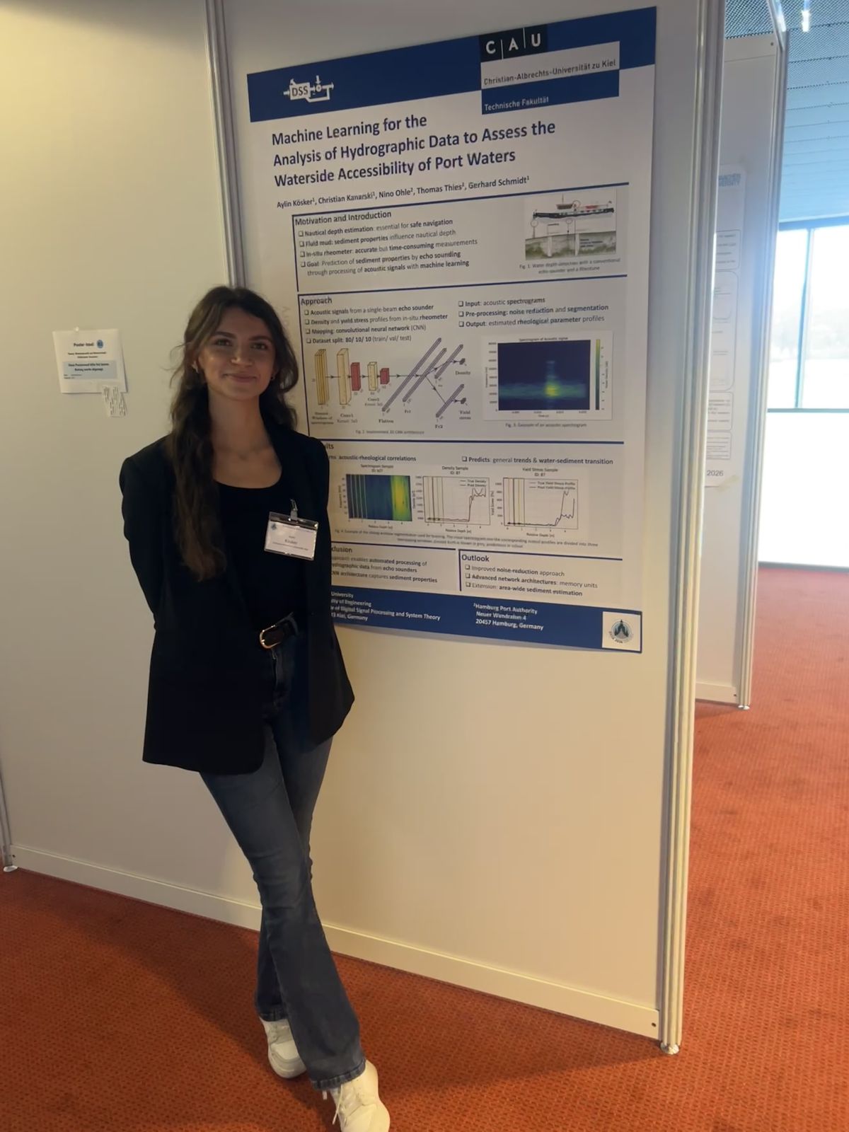 In March 2026, the DSS Chair attended the annual DAGA conference in Dresden. Thanks to the support of the GaS-Club, the student Aylin Kösker was given the opportunity to accompany the chair and participate in the conference from March 23rd to March 26th. As part of the daily poster sessions, she presented the results of her bachelor’s thesis “Machine Learning for the Analysis of Hydrographic Data to Assess the Waterside Accessibility of Port Waters” in the field of Underwater Acoustics. The thesis forms an important basis for an ongoing university research project on the acoustic analysis of sediment properties in harbor areas. The poster session enabled valuable discussions with researchers and conference participants from related research fields.