Lecture "Signals and Systems I"
| Basic Information | |
|---|---|
| Lecturers: | Gerhard Schmidt (lecture), Konstantinos Karatziotis and Ralf Burgardt (exercise) |
| Room: | ES21/Building D - EG.005 (HS I) |
| E-mail: | |
| Language: | German |
| Target group: | Students in electrical engineering and computer engineering |
| Prerequisites: | Mathematics for engineers I, II & III; Foundations in electrical engineering I & II |
| Contents: |
This course teaches basics in systems theory for electrical engineering and information technology. This basic course is restricted to continuous and deterministic signals and systems. Topic overview:
|
| References: | H.W. Schüßler: Netzwerke, Signale und Systeme II: Theorie kontinuierlicher und diskreter Signale und Systeme, Springer, 1991 H.D. Lüke: Signalübertragung, Springer, 1995 |
News
There will be no lecture on June, 15th.
To compensate for that, we will start in the last three weeks earlier, at 08:15 h, with the lecture. This affects the following dates:
- 22.06.2026, start at 08:15 h,
- 29.06.2026, start at 08:15 h,
- 06.07.2026, start at 08:15 h.
Lecture Slides
| Link | Content |
|---|---|
| Slides of the lecture "Introduction" (details of the lecture, notation, signals, systems) |
|
| Slides of the lecture "Signals" (basic signals, reaction on basic signals, signal decomposition) |
|
| Slides of the lecture "Spectral Representations - Part 1" (Fourier series, Discrete Fourier Transform) |
|
| Slides of the lecture "Spectral Representations - Part 2" (Fourier Transform) |
|
| Slides of the lecture "Spectral Representations - Part 3" (Laplace and z-transform) |
|
| Slides of the lecture "Linear Systems" (Basics and relations between different system descriptions) |
|
| Slides of the lecture "Modulation" (Basics and linear modulation schemes) |
Lecture Script
A script for the lecture is available here. It is currently under construction, but a first version is already available via the link mentioned before. If you find some error, please let me (Gerhard Schmidt) know.
Lecture Videos
| Video | Content |
|---|---|
|
Introduction - part 1 of 3 |
|
|
Introduction - part 2 of 3 |
|
|
Introduction - part 3 of 3 |
|
|
Signals - part 1 of 3 |
|
|
Signals - part 2 of 3 |
|
|
Signals - part 3 of 3 |
|
|
Spectra, Fouier series and DFT - part 1 of 3 |
|
|
Spectra, Fouier series and DFT - part 2 of 3 |
|
|
Spectra, Fouier series and DFT - part 3 of 3 |
|
|
Spectra, Fouier transformations - part 1 of 3 |
|
|
Spectra, Fouier transformations - part 2 of 3 |
|
|
Spectra, Fouier transformations - part 3 of 3 |
|
|
Spectra, z and Laplace transform - part 1 of 3 |
|
|
Spectra, z and Laplace transform - part 2 of 3 |
|
|
Spectra, z and Laplace transform - part 3 of 3 |
|
|
Linear systems - part 1 of 4 |
|
|
Linear systems - part 2 of 4 |
|
|
Linear systems - part 3 of 4 |
|
|
Linear systems - part 4 of 4 |
|
|
Modulation - part 1 of 1 |
Exercises
| Date | Event |
|---|---|
| No exercise | |
| No exercise | |
| 30.04.2026 | Theory: Matlab/Python introduction and system properties |
| 07.05.2026 | Question time: Prepare exercises 1 and 2! |
| No exercise (public holiday) | |
| 21.05.2026 | Theory: Perdiodicity and Fourier series | 28.05.2026 | Question time: Prepare exercises 5, 6, 7 and 9! |
| 04.06.2026 | Theory: DFT and Fourier transform |
| 11.06.2026 | Question time: Prepare exercises 11, 12, 14, 15 and 16! |
| 18.06.2026 | Theory: Convolution |
| 25.06.2026 | Question time: Prepare exercises 18, 19 and 21! |
| 02.07.2026 | Theory: Z transform and Laplace transform |
| 09.07.2026 | Question time: Prepare exercises 23, 27, 28 and 31! |
| 09.09.2026 | Exam preparation |
Exercises and Solutions
| Link | Content |
|---|---|
| All exercises. | |
| Solutions to all exercises. |
Exercise Videos
| Video | Content | |
|---|---|---|
|
Exercise 1 |
||
|
Exercise 2 |
||
|
Exercise 3 |
Optional exercise |
|
|
Exercise 4 |
Optional exercise |
|
|
Exercise 5 |
||
|
Exercise 6 |
||
|
Exercise 7 |
||
|
Exercise 8 |
Optional exercise |
|
|
Exercise 9 |
||
|
Exercise 10 |
Optional exercise |
|
|
Exercise 11 |
||
|
Exercise 12 |
||
|
Exercise 13 |
Optional exercise |
|
|
Exercise 14 |
||
|
Exercise 15 |
||
|
Exercise 16 |
||
|
Exercise 17 |
Optional exercise |
|
|
Exercise 18 |
||
|
Exercise 19 |
||
|
Exercise 20 |
Optional exercise |
|
|
Exercise 21 |
||
|
Exercise 22 |
Optional exercise |
|
|
Exercise 23 |
||
|
Exercise 24 |
Optional exercise |
|
|
Exercise 25 |
||
|
Exercise 26 |
Optional exercise |
|
|
Exercise 27 |
||
|
Exercise 28 |
||
|
Exercise 29 |
Optional exercise |
|
|
Exercise 30 |
||
|
Exercise 31 |
||
|
Exam preparation (exam of winter term 2017/2018) |
|
|
|
Exam preparation (exam of winter term 2020/2021) |
|
Matlab Theory Examples
How to use Matlab as a student:
- Campus-wide license (recommended)
- Windows Remote Server
Matlab introduction (click to expand)
close all              % Close all plots
clear                   % Clear workspace
clc                      % Clear console

% Latex font
set(groot, 'DefaultTextInterpreter', 'LaTeX');
set(groot, 'DefaultAxesTickLabelInterpreter', 'LaTeX');
set(groot, 'DefaultAxesFontName', 'LaTeX');
set(groot, 'DefaultAxesFontSize', 14);
set(groot, 'DefaultLegendInterpreter', 'LaTeX');
cmap = lines;

% Get info from matlab docu e.g for command 'close' -------------
% help close % Short overview
% doc close  % Detailed documentation

% Matrix and element wise arithmetic operation -----------------------
% Use ; to suppress output of statement
% a = [1, 2, 3, 4];    % Row vector
% a = [1 2 3 4];       % Same row vector
% b = [2; 3; 4; 5];    % Column vector
% a = a';                 % Transpose vector
% c = b * a;             % Matrix multiplication
% c = a.* a;             % Element wise multiplication


%**************************************************************************
% Basic parameters
%**************************************************************************
f_s = 100;            % Sample rate in Hz
T = 10;                 % Signal duration in s
f_0 = 0.5;             % Test signal frequency in Hz
L = f_s * T;           % Signal length in samples

%**************************************************************************
% Generate signals
%**************************************************************************
% Generate equidistant time scale from 0 to 10 s
t = (0 : L - 1) / f_s;
% Generate sine test signal with frequency f_0
v = sin(2*pi*f_0*t);

%**************************************************************************
% Create plots
%**************************************************************************

%%
% Minimal plot of test signal ----------------------------------------------
figure            % Open new figure
plot(t, v)        % Actual plotting operation

%%
% Plot with some beautification--------------------------------------------
figure
plot(t, v, 'LineWidth', 2, 'Color', 'red')
title('Test signal with some beautification')
xlabel('Time (s)')          % X axis label
ylabel('Magnitude (a.u.)')      % Y axis label
legend('Test signal')    % Add legend
grid on                        % Add legend
xlim([0 1/f_0])              % Limit x-axis to one period

%%
% Discrete stem plot ------------------------------------------------------
figure
stem(t, v)
title('Test signal with stem plot')
xlabel('Time (s)')          % X axis label
ylabel('Magnitude (a.u.)')      % Y axis label
legend('Test signal')    % Add legend
grid on                        % Add legend
xlim([0 0.5])                 % Limit x-axis


%%
% Multiple plots with hold on ----------------------------------------------
figure
plot(t, v)
title('Multiple plots with hold on')
hold on                 % Keep previous plot
plot(t, -v)
xlabel('Time (s)')
ylabel('Magnitude (a.u.)')
legend('Test signal', 'Inv. test signal')
grid on
xlim([0 1/f_0])

%%
% Multiple plots with subplot ----------------------------------------------
% 2 vertical,1 horizontal plot
figure
subplot(2, 1, 1)    % First subplot
plot(t, v)
title('Multiple plots with subplot')
ylabel('Magnitude (a.u.)')
legend('Test signal')
grid on
xlim([0 1/f_0])

subplot(2, 1, 2)    % Second subplot
plot(t, -v)
xlabel('Time (s)')
ylabel('Magnitude (a.u.)')
legend('Inv. test signal')
grid on
xlim([0 1/f_0])

%**************************************************************************
% 3D Plots (will be discussed next week)
%**************************************************************************

%%
% Plot v, v_2 and v_3 as 3D trajectory ----------------------------------

% Generate sine signal as first component
v_x = sin(2*pi*f_0*t).*t;
% Generate cosine signal as second component
v_y = cos(2*pi*f_0*t).*t;
% Generate linear function as third component
v_z = t;

figure
plot3(v_x, v_y, v_z)              % 3D plot
title('3D plot as trajectory')
xlabel('X (m)')
ylabel('Y (m)')
zlabel('Z (m)')
axis image                           % Proportional axis
grid on
%%
% Plot noise as surface plot ----------------------------------------------

% Generate gaussian noise as 2D matrix
L_2 = 50;                              % Use less samples
v_2d = randn(L_2, L_2);        % Generate noise
x =  1 : L_2;                           % X axis
y =  1 : L_2;                           % Y axis

% Surface plot
figure
subplot(2, 1, 1)
surf(x, y, v_2d, 'EdgeColor', 'none', 'FaceColor', 'interp')
title('Surface plot 3D')
c = colorbar;                     % Use colorbar
ylabel(c, 'Magnitude (a.u.)', 'Interpreter', 'latex')
colormap jet
xlabel('X (m)')
ylabel('Y (m)')
zlabel('Z (m)')

subplot(2, 1, 2)
surf(x, y, v_2d, 'EdgeColor', 'none', 'FaceColor', 'interp')
title('Surface plot topview')
c = colorbar;
ylabel(c, 'Magnitude (a.u.)', 'Interpreter', 'latex')
xlabel('X (m)')
ylabel('Y (m)')
zlabel('Z (m)')
view(0, 90)                        % Rotate view to XY
axis tight
System properties demo (click to expand)
close all hidden
clear
clc

set(groot, 'DefaultTextInterpreter', 'LaTeX');
set(groot, 'DefaultAxesTickLabelInterpreter', 'LaTeX');
set(groot, 'DefaultAxesFontName', 'LaTeX');
set(groot, 'DefaultAxesFontSize', 14);
set(groot, 'DefaultLegendInterpreter', 'LaTeX');
cmap = lines;

%**************************************************************************
% Basic parameters
%**************************************************************************
N = 10; % Number of samples

%**************************************************************************
% Calculate support variables and signals
%**************************************************************************
n = (0 : N - 1)';  % Time index

% v -----------------------------------------------------------
v = zeros(N, 1);   % Input signal
v(3) = 2;
v(5) = 0.5;
v(8) = 3;

% y1 -----------------------------------------------------------
y_1 = v;

% y2 -----------------------------------------------------------
% y3 = 2*v(n) + v(n - 1)
y_2 = 2*v;
y_2(2 : end) = y_2(2 : end) + v(1 : end - 1);

% y3 -----------------------------------------------------------
y_3 = 0.5*v + 0.1*n;

% y4 -----------------------------------------------------------
y_4 = zeros(N, 1);
y_4(1 : end - 1) = v(2 : end);

% y5 -----------------------------------------------------------
y_5 = v.^2;

% y6 -----------------------------------------------------------
y_6 = 2*v + 1;

%%
%**************************************************************************
% Plots
%**************************************************************************
% Evaluate section by section to get plots after each other

% Input signal -----------------------------------------------------
figure
% set(gcf, 'Position', [2000 0 1400 1400]) % Set window size

subplot(4, 1, 1)
stem(n, v, 'LineWidth', 2)
grid on
xlabel('\(n\)', 'FontSize', 20);
ylabel('\(v(n)\)', 'FontSize', 20);
grid on
title('Input signal  \(v(n)\)', 'FontSize', 20)

%%
% Complex output signal of system 1 ---------------------------------------
subplot(4, 1, 2)
stem(n, y_1, 'LineWidth', 2, 'Color', cmap(2, :))
hold on
stem(n, zeros(N, 1), 'LineWidth', 2, 'Color', cmap(3, :))
legend({'\(\Re\big\{y_1(n)\big\}\)', '\(\Im\big\{y_1(n)\big\}\)'}, 'FontSize', 20)
grid on
xlabel('\(n\)', 'FontSize', 20);
ylabel('\(y_1(n)\)', 'FontSize', 20);
title('1st system: Output signal \(y_1(n)\)', 'FontSize', 20)

%%
% Output signal of system 2 -----------------------------------------------
subplot(4, 1, 3)
stem(n, y_2, 'LineWidth', 2, 'Color', cmap(4, :))
grid on
xlabel('\(n\)', 'FontSize', 20);
ylabel('\(y_2(n)\)', 'FontSize', 20);
title('2nd: Output signal \(y_2(n)\)', 'FontSize', 20)

%%
% Output signal of system 3 -----------------------------------------------
subplot(4, 1, 4)
stem(n, y_3, 'LineWidth', 2, 'Color', cmap(5, :))
grid on
xlabel('\(n\)', 'FontSize', 20);
ylabel('\(y_3(n)\)', 'FontSize', 20);
title('3rd system: Output signal \(y_3(n)\)', 'FontSize', 20)

%%
figure

% Input signal -----------------------------------------------------
subplot(4, 1, 1)
stem(n, v, 'LineWidth', 2)
grid on
xlabel('\(n\)', 'FontSize', 20);
ylabel('\(v(n)\)', 'FontSize', 20);
grid on
title('Input signal  \(v(n)\)', 'FontSize', 20)

%%
% Output signal of system 4 -----------------------------------------------
subplot(4, 1, 2)
stem(n, zeros(N, 1), 'LineWidth', 2, 'Color', cmap(2, :))
hold on
stem(n, y_4, 'LineWidth', 2, 'Color', cmap(3, :))
grid on
xlabel('\(n\)', 'FontSize', 20);
ylabel('\(y_4(n)\)', 'FontSize', 20);
legend({'\(\Re\big\{y_1(n)\big\}\)', '\(\Im\big\{y_1(n)\big\}\)'}, 'FontSize', 20)
title('4th system: Output signal \(y_4(n)\)', 'FontSize', 20)

%%
% Output signal of system 5 -----------------------------------------------
subplot(4, 1, 3)
stem(n, y_5, 'LineWidth', 2, 'Color', cmap(4, :))
grid on
xlabel('\(n\)', 'FontSize', 20);
ylabel('\(y_5(n)\)', 'FontSize', 20);
title('5th system: Output signal \(y_5(n)\)', 'FontSize', 20)

%%
% Output signal of system 6 -----------------------------------------------
subplot(4, 1, 4)
stem(n, y_6, 'LineWidth', 2, 'Color', cmap(5, :))
grid on
xlabel('\(n\)', 'FontSize', 20);
ylabel('\(y_6(n)\)', 'FontSize', 20);
title('6th system: Output signal \(y_6(n)\)', 'FontSize', 20)
Periodicity demo (click to expand)
close all hidden
clear
clc

set(groot, 'DefaultTextInterpreter', 'LaTeX');
set(groot, 'DefaultAxesTickLabelInterpreter', 'LaTeX');
set(groot, 'DefaultAxesFontName', 'LaTeX');
set(groot, 'DefaultAxesFontSize', 14);
set(groot, 'DefaultLegendInterpreter', 'LaTeX');
cmap = lines;

%**************************************************************************
% Basic paramters
%**************************************************************************
f_s_h = 100;    % Sampling freq for "continuous" signal in Hz
T_0 = 4;          % Fundamental period for normalization in s
f_1 = 1;           % Fundamental freq for sin signal in Hz
T_max = 8;      % Signal duration in seconds

%**************************************************************************
% Calculate support variables
%**************************************************************************
% Continuous signal --------------------------------------
N_h = T_max * f_s_h + 1;    % Duration in samples
t_h = linspace(0, T_max / T_0, T_max * f_s_h + 1); % Time scale in seconds

%**************************************************************************
% Signal selection (uncomment a single signal to use)
%**************************************************************************
% Single cos signal ---------------------------------------
v = cos(2*pi*f_1*t_h);

% Multi cos signal -----------------------------------------
% v = cos(2*pi*f_1*t_h) + cos(2*pi*2*f_1*t_h);

% Rect signal -----------------------------------------------
% v = ones(N_h, 1);
% v(ceil(N_h/2) : end) = v(ceil(N_h/2) : end) * -1;

%**************************************************************************
% Plots
%**************************************************************************
% Evaluate section by section to get plots after each other

figure
% set(gcf, 'Position', [2000 0 1400 1350]) % Set window size

subplot(2, 1, 1)
plot(t_h, v, 'LineWidth', 1)
hold on
grid on
xlabel('\(\frac{t}{T_0}\)', 'FontSize', 30);
ylabel('\(v(t)\)', 'FontSize', 20);
title('Continuous signal  \(v(t)\)', 'FontSize', 20)
%%
% Periodicity check ---------------------------------------
T_p = 1 * T_0;

plot([0 T_p / T_0], [0.01 0.01], 'LineWidth', 3, 'Color', cmap(3, :))
legend('Cont. signal', 'Periodicity')
%%
% Highest frequency check -----------------------------
T_n = 1 * T_0;

plot([0 T_n / T_0], [-0.01 -0.01], 'LineWidth', 3, 'Color', cmap(4, :))
legend('Cont. signal', 'Periodicity', 'Highest freq. component')

%%
% Sampling -------------------------------------------------
T_s = 0.125 * T_0;
t_s = downsample(t_h, f_s_h * T_s);
u = downsample(v, f_s_h * T_s);
N_1 = length(t_s);
n_1 = 0 : N_1 - 1;

stem(t_s, u, 'LineWidth', 2, 'Color', cmap(2, :), 'LineWidth', 2)
legend('Cont. signal', 'Periodicity', 'Highest freq. component', 'Sampling points')

%%
% Reconstruction using SI interpolation ------------
y_1 = zeros(N_h, 1);

r = T_0 / T_s;
t_n = t_h * r;

for i = 0 : N_1 - 1
    y_1 = y_1 + sinc((t_n - i))' * u(i + 1);
end

subplot(2, 1, 2)
stem(n_1, u, 'LineWidth', 2, 'Color', cmap(2, :))
hold on
plot(t_n, y_1)
grid on
xlabel('\(n\)', 'FontSize', 20);
ylabel('\(u(n)\)', 'FontSize', 20);
title('Discrete signal  \(u(n)\)', 'FontSize', 20)
legend('Discrete signal', 'Reconstruction')
Fourier series demo (click to expand)
close all hidden
clear
clc

set(groot, 'DefaultTextInterpreter', 'LaTeX');
set(groot, 'DefaultAxesTickLabelInterpreter', 'LaTeX');
set(groot, 'DefaultAxesFontName', 'LaTeX');
set(groot, 'DefaultAxesFontSize', 14);
set(groot, 'DefaultLegendInterpreter', 'LaTeX');
cmap = lines;

%**************************************************************************
% Basic paramters
%**************************************************************************
f_s_h = 200;    % Sampling freq for "continuous" signal in Hz
T_0 = 4;          % Fundamental period for normalization in s
T_max = 4;      % Signal duration in seconds

%**************************************************************************
% Calculate support variables
%**************************************************************************
% Continuous signal --------------------------------------
N_h = T_max * f_s_h + 1;    % Duration in samples
t_h = linspace(0, T_max / T_0, T_max * f_s_h + 1); % Time scale in seconds

%**************************************************************************
% Signal generation
%**************************************************************************

% Rect signal -----------------------------------------------
v = ones(N_h, 1);
v(ceil(N_h/2) : end) = v(ceil(N_h/2) : end) * -1;

% Fourier series approximation
y = zeros(N_h, 1);

% Number of trigonometric coefficients
M = 10;

% Offset
c_0 = 0;

% Even coefficients
a = zeros(M, 1);

% Odd coefficients
b = zeros(M, 1);

% Calculate odd coefficients according to equation
% b_mu = (4 * h) / (pi * mu)
% Also calculate limited Fourier series approx
for mu = 1 : M
    if mod(mu, 2)
        b(mu) = (4*1) / (pi * mu);
        y = y + b(mu) * sin(2*pi*mu*t_h)';
    else
        b(mu) = 0;
    end
end

% Calculate complex coefficients from trigonometric ones
% c_mu = 1/2 * (a_mu + j * b_mu) with c(-mu) = c(mu)*
c = 1/2 * ([flip(a); c_0; a] + 1i*[-flip(b); 0; b]);

%**************************************************************************
% Plots
%**************************************************************************
% Evaluate section by section to get plots after each other

figure
% set(gcf, 'Position', [2000 0 1400 1350]) % Set window size


subplot(3, 1, 1)
plot(t_h, v, 'LineWidth', 2)
hold on
grid on
xlabel('\(\frac{t}{T_0}\)', 'FontSize', 30);
ylabel('\(v(t)\)', 'FontSize', 20);
title('Continuous rect signal', 'FontSize', 20)

%%
plot(t_h, y, 'LineWidth', 2);
legend('Original signal', 'Finite Fourier series approx.', 'FontSize', 20)

subplot(3, 1, 2)
stem(0, c_0, 'LineWidth', 2)
hold on
stem(a, 'LineWidth', 2)
stem(b, 'LineWidth', 2)
grid on
xlim([0 max(10, M)])
xlabel('\(\mu\)', 'FontSize', 20);
ylabel('\(a_\mu\), \(b_\mu\)', 'FontSize', 25);
title(['Trigonometric Fourier coefficients (\(\mu \leq\) ', num2str(M), ')'], 'FontSize', 20)
legend({'\(c_0 = \frac{a_0}{2}\)', '\( a_\mu\)', '\( b_\mu\)'}, 'FontSize', 20)

%%
subplot(3, 1, 3)
stem(-M : M, real(c), 'LineWidth', 2)
hold on
stem(-M : M, imag(c), 'LineWidth', 2)
grid on
xlim([-max(10, M) max(10, M)])
xlabel('\(\mu\)', 'FontSize', 20);
ylabel('\(c_\mu\)', 'FontSize', 25);
title(['Complex Fourier coefficients (\(\mu \leq\) ', num2str(M), ')'], 'FontSize', 20)
legend({'\(\Re\big\{c_\mu\big\}\)', '\(\Im\big\{c_\mu\big\}\)'}, 'FontSize', 20)
Discrete Fourier transform demo (click to expand)
close all hidden
clear
clc

set(groot, 'DefaultTextInterpreter', 'LaTeX');
set(groot, 'DefaultAxesTickLabelInterpreter', 'LaTeX');
set(groot, 'DefaultAxesFontName', 'LaTeX');
set(groot, 'DefaultAxesFontSize', 14);
set(groot, 'DefaultLegendInterpreter', 'LaTeX');
cmap = lines;

%**************************************************************************
% Basic paramters
%**************************************************************************
f_s = 10;
f_s_h = 200;    % Sampling freq for "continuous" signal in Hz
T_0 = 4;          % Fundamental period for normalization in s
f_1 = 1;           % Fundamental freq for sin signal in Hz
T_max = 4;      % Signal duration in seconds

%**************************************************************************
% Calculate support variables
%**************************************************************************
% Discrete signal --------------------------------------
N = T_max * f_s + 1;                             % Duration in samples
n = 0 : N - 1;                                         % Time indices
mu = -floor((N - 1) / 2) : floor((N - 1) / 2);  % Spectral indices
mu_abs = 0 : floor((N - 1) / 2);                % One-sided spectral indices
%**************************************************************************
% Signal generation
%**************************************************************************

% Unity impulse -----------------------------------------------
% v = zeros(N, 1);
% v(1) = 1;

% Offset ---------------------------------------------------------
v = ones(N, 1);

% Sine signal ------------------------------------------------
% m = 1;
% h = 0;
% v = sin(2*pi*m/N * n) + h;

% Rect signal ------------------------------------------------
% v = ones(N, 1);
% v(n > N / 2) = -v(n > N/2);
% v(1) = 0;


% Compute DFT / FFT
V = fftshift(fft(v) / N);

% Compute one-sided spectrum
V_abs = abs(V(mu >= 0));
V_abs(mu_abs > 0) = 2 * V_abs(mu_abs > 0);

%**************************************************************************
% Plots
%**************************************************************************
% Evaluate section by section to get plots after each other

figure
% set(gcf, 'Position', [2000 0 1400 1350]) % Set window size

subplot(3, 1, 1)
stem(n, v, 'LineWidth', 2)
hold on
grid on
xlabel('\(n\)', 'FontSize', 20);
ylabel('\(v(n)\)', 'FontSize', 20);
title('Discrete signal', 'FontSize', 20)

%%

subplot(3, 1, 2)
stem(mu, real(V), 'LineWidth', 2)
hold on
stem(mu, imag(V), 'LineWidth', 2)
grid on
xlabel('\(\mu\)', 'FontSize', 20);
ylabel('\(V(\mu)\)', 'FontSize', 20);
title('DFT spectrum', 'FontSize', 20)
legend({'\(\Re\big\{V(\mu)\big\}\)', '\(\Im\big\{V(\mu)\big\}\)'}, 'FontSize', 20)

%%
subplot(3, 1, 3)
stem(mu_abs, V_abs, 'LineWidth', 2)
grid on
xlabel('\(\mu\)', 'FontSize', 20);
ylabel('\(|V(\mu)|\)', 'FontSize', 20);
title('One-sided DFT spectrum', 'FontSize', 20)
Fourier transform demo (click to expand)
close all hidden
clear
clc

set(groot, 'DefaultTextInterpreter', 'LaTeX');
set(groot, 'DefaultAxesTickLabelInterpreter', 'LaTeX');
set(groot, 'DefaultAxesFontName', 'LaTeX');
set(groot, 'DefaultAxesFontSize', 14);
set(groot, 'DefaultLegendInterpreter', 'LaTeX');
cmap = lines;

%**************************************************************************
% Basic parameters
%**************************************************************************
f_s = 200;        % Sampling freq for "continuous" signal in Hz
T_0 = 2;          % Fundamental period for signal description in s
T_max = 100;      % Signal duration in seconds

%**************************************************************************
% Calculate support variables
%**************************************************************************
N = T_max * f_s + 1;                     % Duration in samples
t = linspace(-T_max/2, T_max/2, N);      % Time scale in s
w = 2 * pi * linspace(-f_s/2, f_s/2, N); % Frequency scale in s^-1

%**************************************************************************
% Signal generation
%**************************************************************************

signalSel = 5;

switch(signalSel)
    case 1
    % Rect signal -----------------------------------------------
    % Set time signal using ones and zeros
    v = ones(N, 1);                 % Fill signal with ones
    v(t < -T_0) = 0 * v(t < -T_0);  % Set signal before rect pulse to 1
    v(t > T_0) = 0 * v(t > T_0);    % Set signal after rect pulse to 0

    % Set discretized Fourier spectrum to sin(x)/x function
    % NaN value at zero is okay here
    V = abs(2 * sin(w * T_0) ./ w);

   % Use sinc (si) function as better alternative
   % Only with dsp toolbox
   %    V = abs(2 * T_0 * sinc(w / pi * T_0));

    % Calculate approx abs Fourier spectrum based on DFT
    V_dft = abs(fftshift(fft(v) / f_s));

    case 2
    % Sinc signal ----------------------------------------------
    % Define auxiliary parameters
    f_0 = 1;
    w_0 = 2 * pi * f_0;

    % Set time signal to sin(x)/x function
    % NaN value at zero is not okay here as
    % it would make the FFT result NaNs only
    v = (sin(w_0 * t)  + eps) ./ (w_0 * t + eps);

    % Use sinc (si) function as better alternative
    % Only with dsp toolbox
    %  v = sinc(w_0 / pi * t);

    % Set discretized Fourier spectrum to rect pulse
    V = pi / w_0 * ones(N, 1);
    V(w < -w_0) = 0 * V(w < -w_0);
    V(w > w_0) = 0 * V(w > w_0);

    % Calculate approx abs Fourier spectrum based on DFT
    V_dft = abs(fftshift(fft(v) / f_s));

    case 3
    % Exp signal ----------------------------------------------
    % Define auxiliary parameters
    alpha = 0.1;

    % Set time signal to exp function for t > 0
    v = zeros(N, 1);
    v(t >= 0) = exp(-alpha * t(t >= 0));

    % Set discretized Fourier spectrum to 1/(a + jw)
    V = abs(1 ./ (alpha + 1i * w));

    % Calculate approx abs Fourier spectrum based on DFT
    V_dft = abs(fftshift(fft(v) / f_s));

    case 4
    % Cos signal ----------------------------------------------
    % Define auxiliary parameters
    f_0 = 1;
    w_0 = 2 * pi * f_0;

    % Set time signal to exp function for t > 0
    v = cos(w_0 * t);

    % Set discretized Fourier spectrum to zero
    V = zeros(N, 1);
    % Find freq index closest to w_0
    [~, w_0_c] = min(abs(w - w_0));
    % Set value of found index to pi
    V(w_0_c) = pi;
    % Find freq index closest to -w_0
    [~, w_0_c] = min(abs(w + w_0));
    % Set value of found index to pi
    V(w_0_c) = pi;

    % Calculate approx abs Fourier spectrum based on DFT
    % Scaling is different here, why?
    V_dft = abs(fftshift(fft(v) /  N * 2 * pi));

    case 5
    % Combined rect signal -----------------------------
    % Define auxiliary parameters
    a = 1;

    % Set signal composed of multiple rect functions
    v = ones(N, 1);                        % Fill signal with ones
    v(t < -T_0) = 0 * v(t < -T_0);     % Set signal to 0 before first rect pulse
    v(t > -T_0) = a * v(t > -T_0);     % Set signal to a from first rect pulse
    v(t > 0) = 2 * v(t > 0);               % Set signal to 2 * a from second rect pulse
    v(t > T_0) = -1/2 * v(t > T_0);    % Set signal to - a from third rect pulse
    v(t > 4*T_0) = 0 * v(t > 4*T_0);  % Set signal to 0 after third rect pulse


    % Fourier transform according to sample solution
    % Using eps to avoid NaN value in the center
    V = a ./ (1i * w + eps) .* (exp(1i*T_0.*w) + 1 - 3 .* exp(-1i*T_0.*w) + exp(-4i*T_0.*w));

    % Alternative approach to get Fourier transform using rect pulses
    % DSP toolbox only
    % V = 1 * a * T_0 * sinc(w / pi * 0.5 * T_0) .* exp(0.5i * w * T_0);
    % V = V +  2 * a * T_0 * sinc(w / pi * 0.5 * T_0) .* exp(-0.5i * w * T_0);
    % V = V -  3 * a * T_0 * sinc(w / pi * 1.5 * T_0) .* exp(-2.5i * w * T_0);

    % Take absolute value
    V = abs(V);

    V_dft = abs(fftshift(fft(v) /  f_s));

end

%**************************************************************************
% Plots
%**************************************************************************
% Evaluate section by section to get plots after each other

w_lim = 20;

figure
set(gcf, 'Position', [2000 0 1400 1350]) % Set window size

subplot(3, 1, 1)
plot(t, v, 'LineWidth', 2, 'Color', cmap(1, :))
hold on
grid on
xlabel('\(t\) / \(\mathrm{s}\)', 'FontSize', 20);
ylabel('\(v(t)\)', 'FontSize', 20);
title('Continuous time signal (discretized)', 'FontSize', 20)

subplot(3, 1, 2)
plot(w, V, 'LineWidth', 2, 'Color', cmap(2, :))
grid on
xlabel('\(\omega\) / \(\mathrm{s^{-1}}\)', 'FontSize', 20);
ylabel('\(|V(j\omega)|\)', 'FontSize', 20);
title('Fourier spectrum (discretized)', 'FontSize', 20)
xlim([-w_lim, w_lim])

subplot(3, 1, 3)
plot(w, V_dft, 'LineWidth', 2, 'Color', cmap(3, :))
grid on
xlabel('\(\omega\) / \(\mathrm{s^{-1}}\)', 'FontSize', 20);
ylabel('\(|V_{\mathrm{dft}}(j\omega)|\)', 'FontSize', 20);
title('Fourier spectrum approx. using DFT', 'FontSize', 20)
xlim([-w_lim, w_lim])
Convolution demo (click to expand)
close all hidden
clear
clc

set(groot, 'DefaultTextInterpreter', 'LaTeX');
set(groot, 'DefaultAxesTickLabelInterpreter', 'LaTeX');
set(groot, 'DefaultAxesFontName', 'LaTeX');
set(groot, 'DefaultAxesFontSize', 14);
set(groot, 'DefaultLegendInterpreter', 'LaTeX');
cmap = lines;

%**************************************************************************
% Basic paramters
%**************************************************************************
f_s = 10;
T_max = 4;      % Signal duration in seconds

%**************************************************************************
% Calculate support variables
%**************************************************************************
% Discrete signal --------------------------------------
N = T_max * f_s + 1;                             % Duration in samples
n = 0 : N - 1;                                         % Time indices
mu = -floor((N - 1) / 2) : floor((N - 1) / 2);  % Spectral indices
mu_abs = 0 : floor((N - 1) / 2);                % One-sided spectral indices

N_c = 2 * N - 1;                                     % Length of conv. singal in samples
n_c = 0 : N_c - 1;                                  % Time indices of conv signal

%**************************************************************************
% Signal generation
%**************************************************************************

% Set v to rect pulse --------------------------------------------
v = zeros(N, 1);
v(1 : 10) = 1;

% Set signal u ----------------------------------------------------
u = zeros(N, 1);
u(1) = 1;               % Unity impulse
% u(10) = 1;             % Shifted unity impulse
% u(1 : 10) = 1;         % Short rect pulse
% u(1 : 15) = 1;         % Long rect pulse

% Compute convolution of v and u -------------------------
y = conv(v, u);

% Compute DFT / FFT
V = fftshift(fft(v) / N);

U = fftshift(fft(u) / N);

Y = fftshift(fft(y(n_c < N) / N));

%**************************************************************************
% Plots
%**************************************************************************
% Evaluate section by section to get plots after each other

figure
% set(gcf, 'Position', [2000 0 1400 1350]) % Set window size

subplot(3, 2, 1)
stem(n, v, 'LineWidth', 2)
hold on
grid on
xlabel('\(n\)', 'FontSize', 20);
ylabel('\(v(n)\)', 'FontSize', 20);
title('Discrete time signal \(v(n)\)', 'FontSize', 20)

%%
subplot(3, 2, 2)
stem(mu, abs(V), 'LineWidth', 2)
grid on
xlabel('\(\mu\)', 'FontSize', 20);
ylabel('\(|V(\mu)|\)', 'FontSize', 20);
title('Abs. DFT spectrum \(|V(\mu)|\)', 'FontSize', 20)

%%
subplot(3, 2, 3)
stem(n, u, 'LineWidth', 2, 'Color', cmap(2, :))
grid on
xlabel('\(n\)', 'FontSize', 20);
ylabel('\(u(n)\)', 'FontSize', 20);
title('Discrete time signal \(u(n)\)', 'FontSize', 20)

%%
subplot(3, 2, 4)
stem(mu, abs(U), 'LineWidth', 2, 'Color', cmap(2, :))
grid on
xlabel('\(\mu\)', 'FontSize', 20);
ylabel('\(|U(\mu)|\)', 'FontSize', 20);
title('Abs. DFT spectrum \(|U(\mu)|\)', 'FontSize', 20)

%%
subplot(3, 2, 5)
stem(n_c, y, 'LineWidth', 2, 'Color', cmap(3, :))
grid on
xlim([0, N - 1])
xlabel('\(n\)', 'FontSize', 20);
ylabel('\(y(n)\)', 'FontSize', 20);
title('Discrete time signal \(y(n)\)', 'FontSize', 20)

%%
subplot(3, 2, 6)
stem(mu, abs(Y), 'LineWidth', 2, 'Color', cmap(3, :))
grid on
xlabel('\(\mu\)', 'FontSize', 20);
ylabel('\(|Y(\mu)|\)', 'FontSize', 20);
title('Abs. DFT spectrum \(|Y(\mu)|\)', 'FontSize', 20)
Laplace transform demo (click to expand)
close all hidden
clear
clc

set(groot, 'DefaultTextInterpreter', 'LaTeX');
set(groot, 'DefaultAxesTickLabelInterpreter', 'LaTeX');
set(groot, 'DefaultAxesFontName', 'LaTeX');
set(groot, 'DefaultAxesFontSize', 14);
set(groot, 'DefaultLegendInterpreter', 'LaTeX');
cmap = lines;

%**************************************************************************
% Basic parameters
%**************************************************************************
f_s = 200;        % Sampling freq for "continuous" signal in Hz
T_0 = 1;          % Fundamental period for signal description in s
T_max = 100;      % Signal duration in seconds

%**************************************************************************
% Calculate support variables
%**************************************************************************
N = T_max * f_s + 1;                     % Duration in samples
t = linspace(-T_max/2, T_max/2, N);      % Time scale in s
w = 2 * pi * linspace(-f_s/2, f_s/2, N); % Frequency scale in s^-1

%**************************************************************************
% Signal generation
%**************************************************************************

signalSel = 1;

switch(signalSel)

    case 1
        % Sin signal with heaviside function ------------------------------
        % Define auxiliary parameters
        sigma = 0.01;
        w_0 = 2 * pi * 1 / T_0;

        % Time domain signal and labels
        v = sin(w_0 * t);
        v(t < 0) = 0;

        t_lim = 2*[-1 1];
        t_ticks = [-2 -1 0 1 2];
        t_labels = {'', '', '0', '\(T_0\)', ''};

        v_ticks = [-1 0 1];
        v_labels = {'-1', '0', '1'};

        % Area of conversion
        s_re = [0 1 1 0];
        s_im = [1 1 -1 -1];

        s_re_labels = {'\(-\infty\)', '', '0', '', '\(\infty\)'};

        % Laplace domain signal and labels
        s_conv = sprintf('\(\mathrm{Re}\{s\} = %.2f \)', sigma);

        w_lim = 2*w_0*[-1 1];
        w_ticks = w_0*[-2 -1 0 1 2];
        w_labels = {'', '\(-\omega_0\)', '0', '\(\omega_0\)', ''};

        V = w_0 ./ (sigma^2 + 1i * 2 * w + w_0^2 - w.^2);
        V = abs(V);
        V_lim = max(V) * [0 1];
        V_ticks = max(V) * [0 1];
        V_labels = {'0', '0.5'};

    case 2
        % Sin signal without heaviside function -------------------------------
        % Define auxiliary parameters
        w_0 = 2 * pi * 1 / T_0;

        % Time domain signal and labels
        v = sin(w_0 * t);

        t_lim = 2*[-1 1];
        t_ticks = [-2 -1 0 1 2];
        t_labels = {'', '', '0', '\(T_0\)', ''};

        v_ticks = [-1 0 1];
        v_labels = {'-1', '0', '1'};

        % Area of conversion
        s_re = [-0.01, -0.01 0.01 0.01];
        s_im = [-1 1 1 -1];

        s_re_labels = {'\(-\infty\)', '', '0', '', '\(\infty\)'};

        % Laplace domain signal and labels
        s_conv = sprintf('\(\mathrm{Re}\{s\} = 0 \)');

        w_lim = 2*w_0*[-1 1];
        w_ticks = w_0*[-2 -1 0 1 2];
        w_labels = {'', '\(-\omega_0\)', '0', '\(\omega_0\)', ''};

        V = zeros(N, 1);
        % Find freq index closest to w_0
        [~, w_0_c] = min(abs(w - w_0));
        % Set value of found index to pi
        V(w_0_c) = 0.5;
        % Find freq index closest to -w_0
        [~, w_0_c] = min(abs(w + w_0));
        % Set value of found index to pi
        V(w_0_c) = 0.5;

        V = abs(V);

        V_lim = max(V) * [0 1];
        V_ticks = max(V) * [0 1];
        V_labels = {'0', '\(\infty\)'};

    case 3
        % Decreasing exp with heaviside function --------------------------
        % Define auxiliary parameters
        alpha = -0.7;
        sigma = 0.6;
        T_h = log(0.5) / alpha;
        w_0 = 2 * pi * 1 / T_0;

        % Time domain signal and labels
        v = exp(alpha*t); % sin(w_0 * t);
        v(t < 0) = 0;

        t_lim = T_h*2*[-1 1];
        t_ticks = T_h* [-2 -1 0 1 2];
        t_labels = {'', '', '0', '\(T_h\)', ''};

        v_ticks = [-1 0 1];
        v_labels = {'-1', '0', '1'};

        % Area of conversion
        s_re = [-0.5, -0.5 1 1];
        s_im = [-1 1 1 -1];

        s_re_labels = {'\(-\infty\)', '\(s_{\infty}\)', '0', '', '\(\infty\)'};

        % Laplace domain signal and labels
        s_conv = sprintf('\(\mathrm{Re}\{s\} = %.1f \)', sigma);

        w_lim = 4*pi/T_h * [-1 1];
        w_ticks = 2*pi/T_h * [-2 -1 0 1 2];
        w_labels = {'', '\(-\frac{2 \pi}{T_h}\)', '0', '\(\frac{2 \pi}{T_h}\)', ''};

        V = 1 ./ (alpha - sigma - 1i*w);
        V = abs(V);

        V_lim = 1.1 * max(V) * [0 1];
        V_ticks = 1.1 * max(V) * [0 1];
        V_labels = {'0', '\(b\)'};

    case 4
        % Increasing exp with heaviside function --------------------------
        % Define auxiliary parameters
        alpha = 0.7;
        sigma = 0.9;
        T_h = log(2) / alpha;
        w_0 = 2 * pi * 1 / T_0;

        % Time domain signal and labels
        v = exp(alpha*t); % sin(w_0 * t);
        v(t < 0) = 0;

        t_lim = T_h*2*[-1 1];
        t_ticks = T_h* [-2 -1 0 1 2];
        t_labels = {'', '', '0', '\(T_d\)', ''};

        v_ticks = [-1 0 1];
        v_labels = {'-1', '0', '1'};

        % Area of conversion
        s_re = [0.5, 0.5 1 1];
        s_im = [-1 1 1 -1];

        s_re_labels = {'\(-\infty\)', '', '0', '\(s_{\infty}\)', '\(\infty\)'};

        % Laplace domain signal and labels
        s_conv = sprintf('\(\mathrm{Re}\{s\} = %.1f \)', sigma);

        w_lim = 4*pi/T_h * [-1 1];
        w_ticks = 2*pi/T_h * [-2 -1 0 1 2];
        w_labels = {'', '\(-\frac{2 \pi}{T_d}\)', '0', '\(\frac{2 \pi}{T_d}\)', ''};

        V = 1 ./ (alpha - sigma - 1i*w);
        V = abs(V);

        V_lim = 1.1 * max(V) * [0 1];
        V_ticks = 1.1 * max(V) * [0 1];
        V_labels = {'0', '\(b\)'};

end

%**************************************************************************
% Plots
%**************************************************************************
% Evaluate section by section to get plots after each other


figure
% set(gcf, 'Position', [2000 0 1400 1350]) % Set window size

f = subplot(3, 1, 1);
plot(t, v, 'LineWidth', 2, 'Color', cmap(1, :))
hold on
grid on
xlabel('\(t\)', 'FontSize', 20);
ylabel('\(v(t)\)', 'FontSize', 20);
title('Continuous time signal', 'FontSize', 20)
xlim(t_lim)
f.XTickLabelMode = 'manual';
f.XTick = t_ticks;
f.XTickLabel = t_labels;

f.YTickLabelMode = 'manual';
f.YTick = v_ticks;
f.YTickLabel = v_labels;


%%
g = subplot(3, 1, 2);
fill(s_re, s_im, cmap(2, :), 'EdgeColor', 'none')
grid on
xlabel('\(\mathrm{Re}\{s\}\)', 'FontSize', 20);
ylabel('\(\mathrm{Im}\{s\}\)', 'FontSize', 20);
title('Area of conversion', 'FontSize', 20)
xlim([-1 1])
ylim([-1 1])

g.XTickLabelMode = 'manual';
g.XTick = [-1 -0.5 0 0.5 1];
g.XTickLabel = s_re_labels;

g.YTickLabelMode = 'manual';
g.YTick = [-1 0 1];
g.YTickLabel = {'\(-\infty\)', '0', '\(\infty\)'};


%%
h = subplot(3, 1, 3);
plot(w, V, 'LineWidth', 2, 'Color', cmap(3, :))
grid on
xlabel('\(\mathrm{Im}\{s\}\)', 'FontSize', 20);
ylabel('\(|V(s)|\)', 'FontSize', 20);
title(['Laplace spectrum (' s_conv ')'], 'FontSize', 20)
xlim(w_lim)
h.XTickLabelMode = 'manual';
h.XTick = w_ticks;
h.XTickLabel = w_labels;

ylim(V_lim)
h.YTickLabelMode = 'manual';
h.YTick = V_ticks;
h.YTickLabel = V_labels;
z-Domain system demo (click to expand)
close all hidden
clear
clc

set(groot, 'DefaultTextInterpreter', 'LaTeX');
set(groot, 'DefaultAxesTickLabelInterpreter', 'LaTeX');
set(groot, 'DefaultAxesFontName', 'LaTeX');
set(groot, 'DefaultAxesFontSize', 14);
set(groot, 'DefaultLegendInterpreter', 'LaTeX');
cmap = lines;

%**************************************************************************
% Basic parameters
%**************************************************************************
f_s = 48e3;          % Sampling freq in Hz

%**************************************************************************
% System characterisation
%**************************************************************************
systemSel = 4;

% All systems are real-valued (partly complex-conj)
switch(systemSel)
    case 1
        % Stable FIR highpass filter
        % Minimal phase
        z = [0.5 + 0.5j, 0.5 - 0.5j]';
        p = [0 0]';
        [b, a] = zp2tf(z, p, 1);
     case 2
        % Instable IIR lowpass/bandpass filter
        % Maximal phase
        z = [-1 + 1i, -1 - 1i]';
        p = [1/sqrt(2) * (1.2 + 1i), 1/sqrt(2) * (1.2 - 1i)]';
        [b, a] = zp2tf(z, p, 1);
    case 3
        % Stable IIR lowpass (Butterworth) filter
        % Mixed phase (implementation-dependent)
        N = 4;
        [b, a] = butter(N, 0.5);
        [z, p, ~] = tf2zpk(b, a);
    case 4
        % Stable FIR highpass filter
        % Linear phase
        z = [1/(2 * sqrt(2)) *[1 + 1i, 1 - 1i], sqrt(2) *[1 + 1i, 1 - 1i]]';
        p = [0 0 0 0]';
        [b, a] = zp2tf(z, p, 1);
end

% Get system from coefficients
H = tf(b, a, f_s);

% Get frequency response from coefficients
[H_f, w] = freqz(b, a, 2^10);
% Norm frequency vector
w = w / pi;

% Get impulse response from system
[h, t_h] = impulse(H);

%**************************************************************************
% Plots
%**************************************************************************
% Evaluate section by section to get plots after each other

figure
% set(gcf, 'Position', [2000 0 1400 1350]) % Set window size

phi = linspace(0, 2*pi, 1000);
x = cos(phi);
y = sin(phi);

% Pole zero plot
subplot(4, 1, 1);
plot(real(z), imag(z), 'LineStyle', 'none', 'Marker', 'o', 'Color', cmap(1, :))
hold on
plot(real(p), imag(p), 'LineStyle', 'none', 'Marker', 'x', 'Color', cmap(1, :))
plot(x, y, '--', 'Color', 'Black')
plot([-4 4], [0 0], '--', 'Color', 'Black')
plot([0 0], [-4 4], '--', 'Color', 'Black')
xlim([-2 2])
ylim([-2 2])
grid on
xlabel('\(\mathrm{Re}\big(z\big)\)')
ylabel('\(\mathrm{Im}\big(z\big)\)')
title('Pole-zero plot')

%%
% Magnitude of frequency response
subplot(4, 1, 2)
plot(w, 20*log10(abs(H_f)))
grid on
xlabel('\(\frac{\Omega}{\pi}\)')
ylabel('\(|H\big(e^{j \Omega}\big)|\) / dB')
title('Frequency response - magnitude')

%%
% Impulse response
subplot(4, 1, 3)
stem(t_h, h)
grid on
xlabel('\(n \, T_s\) / s')
title('Impulse response')

%%
% Phase of frequency response
subplot(4, 1, 4)
plot(w, rad2deg(unwrap(angle(H_f))))
grid on
xlabel('\(\frac{\mathrm{\Omega}}{\pi}\)')
ylabel('\(\phi\) / deg')
title('Frequency response - phase')
Python Theory Examples
Python introduction (click to expand)
import numpy as np # python extension for vector and matrix operations
import matplotlib.pyplot as plt # python extension for plotting

# Matrix and element wise arithmetic operation ---------------------------------------------
a = np.array([[1,2,3,4]])         # Row vector
b = np.array([[2],[3],[4],[5]])   # Column vector
a = a.T              # Transpose vector
a = np.transpose(a)  # Second way transpose vector
c = np.matmul(b,a)   # Matrix multiplication
c = np.multiply(a,a) # Element wise multiplication

#**************************************************************************
# Basic parameters
#**************************************************************************
f_s = 100.;            # Sample rate in Hz
T   = 10.0             # Signal duration in s
f_0 = 0.5              # Test signal frequency in Hz
L   = int(f_s * T)     # Signal length in samples

#**************************************************************************
# Generate signals
#**************************************************************************
# Generate equidistant time scale from 0 to 10 s
t = np.arange(0,L, dtype=float) / f_s
# Generate sine test signal with frequency f_0
v = np.sin(2*np.pi*f_0*t);

#**************************************************************************
# Create plots
#**************************************************************************
# Minimal plot of test signal
plt.figure()
plt.plot(t,v)
plt.show()

# Plot with some beautification ------------------------------------------
plt.figure
plt.plot(t,v, linewidth=2, color='red')
plt.title('Test signal with some beautification')
plt.xlabel('Time /s')
plt.ylabel('Test signal')
plt.xlim((0, 1/f_0))
plt.grid()
plt.show()

# Discrete stem plot ------------------------------------------------------
plt.figure()
plt.stem(t,v, basefmt=" ")
plt.title("Test signal with stem plot")
plt.xlabel('Time /s')
plt.ylabel('Magntiude')
plt.legend(['Test signal'])
plt.xlim((0,0.5))
plt.ylim((0,1))
plt.grid()
plt.show()

# Multiple plots ----------------------------------------------------------
plt.figure()
plt.plot(t,v)
plt.plot(t,-v)
plt.xlabel('Time / s')
plt.ylabel('Magnitude')
plt.legend(['Test signal', 'Inv. test signal'])
plt.grid()
plt.xlim((0,1/f_0))
plt.show()

# Multiple plots with subplot --------------------------------------------
# 2 vertical, 1 horizontal plot
fig, ax = plt.subplots(2,1)  # First subplot
ax[0].plot(t, v)
ax[0].set_title('Multiple plots with subplot')
ax[0].set_ylabel('Magnitude')
ax[0].legend(['Test signal'])
ax[0].grid()
ax[0].set_xlim((0,1/f_0))

# Second subplot
ax[1].plot(t, -v)
ax[1].set_xlabel('Time / s')
ax[1].set_ylabel('Magnitude')
ax[1].legend(['Inv. test signal'])
ax[1].grid()
ax[1].set_xlim((0, 1/f_0))
plt.show()

#**************************************************************************
# 3D Plots (will be discuessed next week)
#**************************************************************************
#
# Plot v, v_2 and v_3 as 3D trajectory ----------------------------------

# Generate sine signal as first component
v_x = np.multiply(np.sin(2*np.pi*f_0*t),t);
# Generate cosine signal as second component
v_y = np.multiply(np.cos(2*np.pi*f_0*t),t);
# Generate linear function as third component
v_z = t

# Create a 3D plot
fig = plt.figure()
ax = fig.add_subplot(111,projection='3d')
ax.plot(v_x,v_y,v_z)
ax.set_title('3D plot as trajectory')
ax.set_xlabel('X / m')
ax.set_ylabel('Y / m')
ax.set_zlabel('Z / m', rotation=0)
ax.zaxis.labelpad=-5
plt.show()

# Plot noise as surface plot
# Generate gaussian noise as 2D matrix
L_2  = 50;                               # Use less samples
v_2d = np.random.randn(L_2, L_2);        # Generate noise
x    = np.arange(0,L_2)                  # X axis
y    = np.arange(0,L_2)                  # Y axis

fig     = plt.figure(figsize=(10,10))

ax1     = fig.add_subplot(211,projection='3d')
x,y     = np.meshgrid(x,y)
surf1   = ax1.plot_surface(x, y, v_2d, linewidth=0, antialiased=False, cmap='jet')
ax1.set_xlabel('X / m')
ax1.set_ylabel('Y / m')
ax1.set_zlabel('Z / m')
ax1.set_title('Surface plot 3D')
cbar1 = fig.colorbar(surf1)
cbar1.set_label('Magnitude')

ax2     = fig.add_subplot(212,projection='3d')
surf2   = ax2.plot_surface(x, y, v_2d, linewidth=0, antialiased=False, cmap='jet')
ax2.set_xlabel('X / m')
ax2.set_ylabel('Y / m')
ax2.set_zlabel('Z / m')
ax2.set_title('Surface plot topview')
ax2.view_init(azim=270, elev=90)
ax.axis('tight')
cbar1   = fig.colorbar(surf2)
cbar1.set_label('Magnitude')
plt.ioff()
plt.show()
System properties demo (click to expand)
import numpy as np              # python extension for vector and matrix operations
import matplotlib.pyplot as plt # python extension for plotting

#**************************************************************************
# Basic paramters
#**************************************************************************
N = 10; # Number of samples

#**************************************************************************
# Calculate support variables and signals
#**************************************************************************
n = np.arange(0,N)  # Time index
n = n.reshape(N,1)
# v -----------------------------------------------------------
v = np.zeros((N, 1));   # Input signal
v[1] = 1
v[4] = 0.5
v[7] = 1

# y1 -----------------------------------------------------------
y_1 = v

# y2 -----------------------------------------------------------
# y3 = 2*v(n) + v(n - 1)
y_2 = 2*v
y_2[1:] = y_2[1:] + v[0 : - 1]

# y3 -----------------------------------------------------------
y_3 = np.zeros((N, 1))
y_3[0:] = 2*v[0:]
y_3 = np.multiply(y_3,n + 1) / 10 + 0.1
#y_3 = y_3.* (n + 1) / 10 + 0.1;

# y4 -----------------------------------------------------------
y_4 = np.zeros((N, 1))
y_4[0 :-1] = v[1 :]

# y5 -----------------------------------------------------------
y_5 = v**2

# y6 -----------------------------------------------------------
y_6 = 2*v + 0.2

#**************************************************************************
# Plots
#**************************************************************************
# Evaluate section by section to get plots after each other
fig, ax = plt.subplots(2,1, figsize=(6,10))
markerline, _, _ = ax[0].stem(n,v,basefmt=' ')
plt.setp(markerline, 'markerfacecolor', 'none')
ax[0].grid()
ax[0].set_xlabel('\(n\)')
ax[0].set_ylabel('\(v(n)\)')
ax[0].set_title('Input signal  \(v(n)\)')

# output signal of system 1 -----------------------------------------------
markerline, stemlines, _ =  ax[1].stem(n, y_1, basefmt=' ')
plt.setp(markerline, 'markerfacecolor', 'none', 'color','red')
plt.setp(stemlines, 'color', 'red')
ax[1].grid()
ax[1].set_xlabel('\(n\)')
ax[1].set_ylabel('\(y_1(n)\)')
ax[1].set_title('1st system: Real output signal \(y_1(n)\)')
plt.show()

fig, ax = plt.subplots(3,1, figsize=(8,15))
markerline0, stemlines0, _ = ax[0].stem(n, np.zeros((N, 1)),basefmt=' ')
markerline1, stemlines1, _ = ax[0].stem(n, y_1,basefmt=' ')
plt.setp(markerline0, 'markerfacecolor', 'none', 'color','red')
plt.setp(stemlines0, 'color', 'red')
plt.setp(markerline1, 'markerfacecolor', 'none', 'color','orange')
plt.setp(stemlines1, 'color', 'orange')
ax[0].legend([r'\(\Re\{y_1(n)\}\)', r'\(\Im\{y_1(n)\}\)'])
ax[0].grid()
ax[0].set_xlabel('\(n\)')
ax[0].set_ylabel('\(y_1(n)\)')
ax[0].set_title('1st system: Complex output signal \(y_1(n)\)')

markerline, stemlines, _ = ax[1].stem(n, y_2, basefmt=' ')
plt.setp(markerline, 'markerfacecolor', 'none', color='purple')
plt.setp(stemlines, color='purple')
ax[1].grid()
ax[1].set_xlabel('\(n\)')
ax[1].set_ylabel('\(y_2(n)\)')
ax[1].set_title('2nd: Output signal \(y_2(n)\)')

markerline, stemlines, _ = ax[2].stem(n, y_3, basefmt=' ')
plt.setp(markerline, 'markerfacecolor', 'none', color='green')
plt.setp(stemlines, color='green')
ax[2].grid()
ax[2].set_xlabel('\(n\)')
ax[2].set_ylabel('\(y_3(n)\)')
ax[2].set_title('3rd system: Output signal \(y_3(n)\)')
plt.show()

fig, ax = plt.subplots(4,1, figsize=(8,20))

# Input signal -----------------------------------------------------
markerline, stemlines, _ = ax[0].stem(n, v, basefmt=' ')
plt.setp(markerline, 'markerfacecolor','none')
ax[0].grid()
ax[0].set_xlabel('\(n\)')
ax[0].set_ylabel('\(v(n)\)')
ax[0].set_title('Input signal  \(v(n)\)')

# Output signal of system 4 -----------------------------------------------
markerline, stemlines, _ = ax[1].stem(n, y_4, basefmt=' ')
plt.setp(markerline, 'markerfacecolor', 'none', color='red')
plt.setp(stemlines, color='red')
ax[1].grid()
ax[1].set_xlabel('\(n\)')
ax[1].set_ylabel('\(y_4(n)\)')
ax[1].set_title('4th system: Output signal \(y_3(n)\)')

# Output signal of system 5 -----------------------------------------------
markerline, stemlines, _ = ax[2].stem(n, y_5, basefmt=' ')
plt.setp(markerline, 'markerfacecolor', 'none', color='orange')
plt.setp(stemlines, color='orange')
ax[2].grid()
ax[2].set_xlabel('\(n\)')
ax[2].set_ylabel('\(y_4(n)\)')
ax[2].set_title('5th system: Output signal \(y_3(n)\)')

# Output signal of system 6 -----------------------------------------------
markerline, stemlines, _ = ax[3].stem(n, y_6, basefmt=' ')
plt.setp(markerline, 'markerfacecolor', 'none', color='green')
plt.setp(stemlines, color='green')
ax[3].grid()
ax[3].set_xlabel('\(n\)')
ax[3].set_ylabel('\(y_4(n)\)')
ax[3].set_title('6th system: Output signal \(y_3(n)\)')
plt.show()
Evaluation
The completed evaluations of the last years can be found here. Please note that this page contains the evaluations of all of our lectures. As a consequence you must scroll down to get to the evaluations of this lecture.
The form for the current evaluation can be started here.
Formulary
A formulary can be found below:
| Link | Content |
|---|---|
| Formulary |
Previous Exams
| Link | Content | Link | Content |
|---|---|---|---|
| Exam of the winter term 2025/2026 | Corresponding solution | ||
| Exam of the summer term 2025 | Corresponding solution | ||
| Exam of the winter term 2024/2025 | Corresponding solution | ||
| Exam of the summer term 2024 | Corresponding solution | ||
| Exam of the winter term 2023/2024 | Corresponding solution |
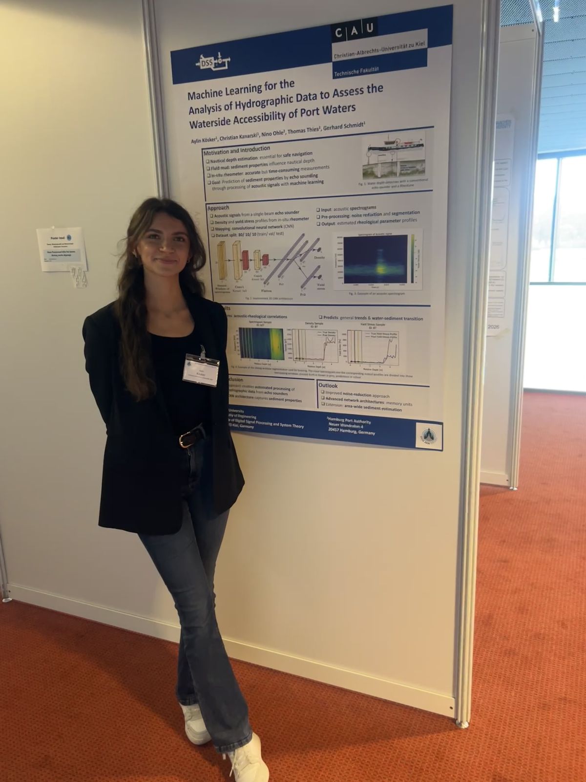 In March 2026, the DSS Chair attended the annual DAGA conference in Dresden. Thanks to the support of the GaS-Club, the student Aylin Kösker was given the opportunity to accompany the chair and participate in the conference from March 23rd to March 26th. As part of the daily poster sessions, she presented the results of her bachelor’s thesis “Machine Learning for the Analysis of Hydrographic Data to Assess the Waterside Accessibility of Port Waters” in the field of Underwater Acoustics. The thesis forms an important basis for an ongoing university research project on the acoustic analysis of sediment properties in harbor areas. The poster session enabled valuable discussions with researchers and conference participants from related research fields.