Lecture "Signals and Systems II"
| Basic Information | |
|---|---|
| Lecturers: | Gerhard Schmidt (lecture), Konstantinos Karatziotis and Ralf Burgardt (exercise) |
| Room: | ES21/Geb.D - EG.004 (HS II) - Heinrich-Hertz-Hörsaal |
| E-mail: | |
| Language: | German |
| Target group: | Students in electrical engineering and computer engineering |
| Prerequisites: | Signals and Systems, Part 1 |
| Contents: |
This course teaches basics in systems theory for electrical engineering and information technology. This basic course is focused on stochastic signals and linear systems. Topic overview:
|
| References: | E. Hänsler: Statistische Signale, 3.Auflage, Springer, 2001 H. D. Lüke: Signalübertragung, Springer, 1995 H. W. Schüßler: Netzwerke, Signale und Systeme II: Theorie kontinuierlicher und diskreter Signale und Systeme, Springer, 1991 |
News
Scroll down to find a list of the topics with a detailed schedule for the exercises in WS25/26.
The exam review for Signals and Systems 2 will take place on Monday, April 20, from 3 PM to 4 PM in Building C, Room 01.028.
Lecture Slides
| Link | Content |
|---|---|
| Slides of the lecture "Modulation" (Linear and nonlinear modulation, digitalization) |
|
| Slides of the lecture "State-space description" (State-space representation of linear, time-invariant systems) |
|
| Slides of the lecture "Stochastic signals and corresponding spectra" (Random processes, power spectral densities) |
|
| Slides of the lecture "Stochastic signals and linear time-invariant systems" (Random processes, power spectral densities) |
|
| Slides of the lecture "Ideal systems" (Lowpass filter, magnitude and phase distortions) |
|
| Slides of the lecture "Extensions on transformations" (Spectra of sampled continuous and discrete signals, convergence conditions and inverse transformations) |
Lecture Videos
| Video | Content |
|---|---|
|
Modulation - part 1 of 2 |
|
|
Modulation - part 2 of 2 |
|
|
State-space description - part 1 of 2 |
|
|
State-space description - part 2 of 2 |
|
|
Random processes - part 1 of 2 |
|
|
Random processes - part 2 of 2 |
|
|
Reaction of linear systems to random processes - part 1 of 1 |
|
|
Ideal systemes - part 1 of 2 |
|
|
Ideal systemes - part 2 of 2 |
|
|
Add-ons (transforms) - part 1 of 2 |
|
|
Add-ons (transforms) - part 2 of 2 |
Lecture Script
A script for the lecture is available here. It is currently under construction, but a first version is already available via the link mentioned before. If you find some error, please let me (Gerhard Schmidt) know.
Exercises
| Date | Event |
|---|---|
| No exercise | |
| 27.10.2025 | Intro, Theory, Amplitude Modulation |
| 03.11.2025 | Question time: Please prepare exercises 1 and 2! |
| 10.11.2025 | Theory: Angle modulation |
| 17.11.2025 | Question time: Please prepare exercises 3 and 4! |
| 25.11.2025 | Theory: Pulse amplitude modulation |
| 01.12.2025 | Theory: State-space description |
| 08.12.2025 | Question time: Please prepare exercise 6! |
| 15.12.2025 | DEMO session at the chair |
| No exercise (Winter break) | |
| No exercise (Winter break) | |
| 05.01.2026 | Theory: Distribution and Correlation |
| 12.01.2026 | Question time: Please prepare exercises 9 and 10! |
| 19.01.2026 | Theory: Correlation and systems |
| 26.01.2026 | Question time: Please prepare exercises 11, 12 and 16! |
| 16.03.2026 | Exam preparation, Room: HS II, Time: 12:30 - 14:00 |
Exercises
| Link | Content |
|---|---|
| All exercises. |
Solutions for the Exercises
| Link | Content |
|---|---|
| Solutions to all exercises. |
Exercise Videos
| Video | Content | Please watch until |
|---|---|---|
|
Exercise 1 |
30.10.2023 |
|
|
Exercise 2 |
30.10.2023 |
|
|
Exercise 3 |
13.11.2023 |
|
|
Exercise 4 |
13.11.2023 |
|
|
Exercise 5 |
27.11.2023 |
|
|
Exercise 6 |
18.12.2024 |
|
|
Exercise 7 |
Optional exercise |
|
|
Exercise 8 |
Optional exercise |
|
|
Exercise 9 |
15.01.2024 |
|
|
Exercise 10 |
15.01.2024 |
|
|
Exercise 11 |
29.01.2024 |
|
|
Exercise 12 |
29.01.2024 |
|
|
Exercise 13 |
Optional exercise |
|
|
Exercise 14 |
Optional exercise |
|
|
Exercise 15 |
Optional exercise |
|
|
Exercise 16 |
29.01.2024 |
|
|
Exam preparation |
|
Matlab Theory Examples
Students can use MATLAB for free on their own devices using the new campus-wide license. Alternatively, students can use Windows Remote Server to run Matlab scripts from home.
Matlab introduction (click to expand)
%**************************************************************************
% Matlab introduction
% SuS II (WS21)
%**************************************************************************

close all              % Close all plots
clear                   % Clear workspace
clc                      % Clear console

% Set all fonts to latex style
set(groot, 'DefaultTextInterpreter', 'LaTeX');
set(groot, 'DefaultAxesTickLabelInterpreter', 'LaTeX');
set(groot, 'DefaultAxesFontName', 'LaTeX');
set(groot, 'DefaultAxesFontSize', 14);
set(groot, 'DefaultLegendInterpreter', 'LaTeX');

% Save color map in variable
cmap = lines;

% Get info from matlab docu e.g for command 'close' -------------
% help close % Short overview
% doc close  % Detailed documentation

% Matrix and element wise arithmetic operations ---------------------
% Use ; to suppress output of statement
% a = [1, 2, 3, 4];    % Row vector
% a = [1 2 3 4];       % Same row vector
% b = [2; 3; 4; 5];    % Column vector
% a = a';                 % Transpose vector
% c = b * a;             % Matrix multiplication
% c = a.* a;             % Element wise multiplication
% size(c)                 % Get matrix dimensions
% length(c)             % Get max of matrix dim.


%**************************************************************************
% Basic parameters
%**************************************************************************
f_s = 100;            % Sample rate [Hz]
T = 10;                 % Signal duration [s]
f_0 = 0.5;             % Test signal frequency [Hz]

%**************************************************************************
% Auxiliary parameters
%**************************************************************************
L = f_s * T + 1;     % Signal length

% Generate equidistant time scale from 0 to 10 s
t = (0 : L - 1) / f_s;

%**************************************************************************
% Generate signals
%**************************************************************************
% Generate sine test signal with frequency f_0
v = sin(2*pi*f_0*t);

% Generate uniformly distributed noise signal
v_u = rand(1, L);

% Generate gaussian noise signal
v_g = randn(1, L);

%**************************************************************************
% Create plots
%**************************************************************************

%%
% Minimal plot of test signal ----------------------------------------------
figure            % Open new figure
plot(t, v_g)        % Actual plotting operation

%%
% Plot with some beautification--------------------------------------------
figure
plot(t, v, 'LineWidth', 2, 'Color', 'red')
title('Test signal with some beautification')
xlabel('Time / s')          % X axis label
ylabel('Magnitude')      % Y axis label
legend('Test signal')    % Add legend
grid on                        % Add legend
xlim([0 1/f_0])              % Limit x-axis to one period

%%
% Discrete stem plot ------------------------------------------------------
figure
stem(t, v)
title('Test signal with stem plot')
xlabel('Time / s')          % X axis label
ylabel('Magnitude')      % Y axis label
legend('Test signal')    % Add legend
grid on                        % Add legend
xlim([0 0.5])                 % Limit x-axis


%%
% Multiple plots with hold on ----------------------------------------------
figure
plot(t, v)
title('Multiple plots with hold on')
hold on                 % Keep previous plot
plot(t, -v)
xlabel('Time / s')
ylabel('Magnitude')
legend('Test signal', 'Inv. test signal')
grid on
xlim([0 1/f_0])

%%
% Multiple plots with subplot ----------------------------------------------
% 2 vertical,1 horizontal plot
figure
subplot(2, 1, 1)    % First subplot
plot(t, v)
title('Multiple plots with subplot')
ylabel('Magnitude')
legend('Test signal')
grid on
xlim([0 1/f_0])

subplot(2, 1, 2)    % Second subplot
plot(t, -v)
xlabel('Time / s')
ylabel('Magnitude')
legend('Inv. test signal')
grid on
xlim([0 1/f_0])

%**************************************************************************
% 3D Plots (will be discussed next week)
%**************************************************************************

%%
% Plot v, v_2 and v_3 as 3D trajectory ----------------------------------

% Generate sine signal as first component
v_x = sin(2*pi*f_0*t).*t;
% Generate cosine signal as second component
v_y = cos(2*pi*f_0*t).*t;
% Generate linear function as third component
v_z = t;

figure
plot3(v_x, v_y, v_z)              % 3D plot
title('3D plot as trajectory')
xlabel('X / m')
ylabel('Y / m')
zlabel('Z / m')
axis image                           % Proportional axis
grid on
%%
% Plot noise as surface plot ----------------------------------------------

% Generate gaussian noise as 2D matrix
L_2 = 50;                              % Use less samples
v_2d = randn(L_2, L_2);        % Generate noise
x =  1 : L_2;                           % X axis
y =  1 : L_2;                           % Y axis

% Surface plot
figure
subplot(2, 1, 1)
surf(x, y, v_2d, 'EdgeColor', 'none', 'FaceColor', 'interp')
title('Surface plot 3D')
c = colorbar;                     % Use colorbar
ylabel(c, 'Magnitude')
colormap jet
xlabel('X / m')
ylabel('Y / m')
zlabel('Z / m')

subplot(2, 1, 2)
surf(x, y, v_2d, 'EdgeColor', 'none', 'FaceColor', 'interp')
title('Surface plot topview')
c = colorbar;
ylabel(c, 'Magnitude')
xlabel('X / m')
ylabel('Y / m')
zlabel('Z / m')
view(0, 90)                        % Rotate view to XY
axis tight
Amplitude modulation (click to expand)
%**************************************************************************
% Amplitude modulation and signal obfuscation
% SuS II (WS21)
%**************************************************************************

close all hidden
clear
clc

set(groot, 'DefaultTextInterpreter', 'LaTeX');
set(groot, 'DefaultAxesTickLabelInterpreter', 'LaTeX');
set(groot, 'DefaultAxesFontName', 'LaTeX');
set(groot, 'DefaultAxesFontSize', 14);
set(groot, 'DefaultLegendInterpreter', 'LaTeX');

%**************************************************************************
% Basic parameters
%**************************************************************************
f_s      = 120e3;        % Sampling frequency in Hz
f_low    = 2e3;        % Lowest signal frequency in Hz
f_high   = 4e3;        % Highest signal frequency in Hz
f_mod1   = 20e3;         % Modulation frequency in Hz
f_mod2   = 25e3;         % Modulation frequency 2 in Hz
T_signal = 10;           % Signal length in s

%**************************************************************************
% Calculate support variables
%**************************************************************************
bw = f_high - f_low;                           % Bandwidth in Hz
L_signal = T_signal * f_s;                     % Signal length in samples
t = (0 : L_signal - 1) / f_s;                  % Time scale
f = linspace(-f_s/2, f_s/2, L_signal)./1e3;    % Frequency scale
v_mod1 = sin(2*pi*f_mod1*t)';                  % Modulation signal
v_mod2 = sin(2*pi*f_mod2*t)';                  % Modulation signal 2

%**************************************************************************
% Design filters
%**************************************************************************
% Design FIR highpass filter (complicated...)

f_hp = f_mod1 + [-1e3, 1e3];
a_hp = [0 1];
rp = 1;
rs = 120;

dev = [(10^(rp/20)-1)/(10^(rp/20)+1)  10^(-rs/20)];
[n_ord_bp,fo_bp,ao_bp,w] = firpmord(f_hp,a_hp,dev,f_s);

b_high = firpm(n_ord_bp+1,fo_bp,ao_bp);


% Design Butterworth lowpass filter for demodulation -----------------------------
f_c = 30e3;      % Cutoff freq in Hz
n = 30;          % Cutoff freq in Hz

[z,p,k] = butter(n, f_c/(f_s/2));
[sos_low, g_low] = zp2sos(z, p, k);

%**************************************************************************
% Generate initial time signal
%**************************************************************************
% Use sum of multiple sine functions in specified frequency range

u = 1* sin(2*pi*f_low*t)';
u = u + 0.5 *sin(2*pi*f_high*t)';
%%
%**************************************************************************
% Processing chain for amplitude modulation
%**************************************************************************
% Modulate, demodulate and filter inital signal
% Use either this or the other processing chains

% Process FFT of initial time signal --------------------------------------
% Process FFT:                  fft(..)
% Absolute spectrum:            abs(..)
% Weight correctly:             ../ L
% Shift to get correct x axis:  circshift(.., - ceil(L / 2)
% See MATLAB docu for more info on FFT processing
U = circshift(abs(fft(u)) / L_signal, - ceil(L_signal/2));

% Modulation step ---------------------------------------------------------
g_1 = u.*v_mod1;
G_1 = circshift(abs(fft(g_1)) / L_signal, - ceil(L_signal/2));

% Demodulation step -------------------------------------------------------
g_2 = g_1.*v_mod1;
G_2 = circshift(abs(fft(g_2)) / L_signal, - ceil(L_signal/2));

% Lowpass filter step -----------------------------------------------------
g_3 = sosfilt(sos_low, g_2);
G_3 = circshift(abs(fft(g_3)) / L_signal, - ceil(L_signal/2));

% Not used ----------------------------------------------------------------
g_4 = zeros(L_signal, 1);
G_4 = zeros(L_signal, 1);

%%
%**************************************************************************
% Processing chain for signal obfuscation
%**************************************************************************
% Modulate, highpass filter, modulate again, lowpass filter
% Insert "u = g_4;" in second turn to reconstruct initial signal

% Process FFT -------------------------------------------------------------
U = circshift(abs(fft(u)) / L_signal, - ceil(L_signal/2));

% Modulation step ---------------------------------------------------------
g_1 = u.*v_mod1;
G_1 = circshift(abs(fft(g_1)) / L_signal, - ceil(L_signal/2));

% Supress lower frequency band --------------------------------------------
%g_2 = sosfilt(sosHigh, g_1);
g_2 = filtfilt(b_high, 1, g_1);
G_2 = circshift(abs(fft(g_2)) / L_signal, - ceil(L_signal/2));

% Modulation step ---------------------------------------------------------
g_3 = g_2.*v_mod2;
G_3 = circshift(abs(fft(g_3)) / L_signal, - ceil(L_signal/2));

% Lowpass filter step -----------------------------------------------------
g_4 = filtfilt(sos_low, g_low, g_3); %filter(b_high, 1, g_3)
G_4 = circshift(abs(fft(g_4)) / L_signal, - ceil(L_signal/2));

%**************************************************************************
% Processing chain for signal obfuscation reversal
%**************************************************************************
% Modulate, highpass filter, modulate again, lowpass filter

% Modulation step ---------------------------------------------------------
g_5 = g_4.*v_mod1;
G_5 = circshift(abs(fft(g_5)) / L_signal, - ceil(L_signal/2));

% Supress lower frequency band --------------------------------------------
g_6 = filtfilt(b_high, 1, g_5);
G_6 = circshift(abs(fft(g_6)) / L_signal, - ceil(L_signal/2));

% Modulation step ---------------------------------------------------------
g_7 = g_6.*v_mod2;
G_7 = circshift(abs(fft(g_7)) / L_signal, - ceil(L_signal/2));

% Lowpass filter step -----------------------------------------------------
g_8 = filtfilt(sos_low, g_low, g_7); %filter(b_high, 1, g_3)
G_8 = circshift(abs(fft(g_8)) / L_signal, - ceil(L_signal/2));

%%
%**************************************************************************
% Plots
%**************************************************************************
% Evaluate section by section to get plots after each other

t_range = 1e-2; % Limited time axis scale is easier to view

figure
set(gcf, 'Position', [2000 0 1400 1400]) % Set window size

subplot(5, 2, 1)
plot(t, u)
xlim([0, t_range])
ylabel('\(u(t)\)')
grid on

subplot(5, 2, 2)
plot(f, U)
ylabel('\(|U_(jw)|\)')
grid on

%%
subplot(5, 2, 3)
plot(t, g_1)
xlim([0, t_range])
ylabel('\(g_\mathrm{1}(t)\)')
grid on

subplot(5, 2, 4)
plot(f, G_1)
ylabel('\(|G_\mathrm{1}(jw)|\)')
grid on

%%
subplot(5, 2, 5)
plot(t, g_2)
xlim([0, t_range])
ylabel('\(g_\mathrm{2}(t)\)')
grid on

subplot(5, 2, 6)
plot(f, G_2)
ylabel('\(|G_\mathrm{2}(jw)|\)')
grid on

%%
subplot(5, 2, 7)
plot(t, g_3)
xlim([0, t_range])
ylabel('\(g_\mathrm{3}(t)\)')
grid on

subplot(5, 2, 8)
plot(f, G_3)
ylabel('\(|G_\mathrm{3}(jw)|\)')
grid on

%%
subplot(5, 2, 9)
plot(t, g_4)
xlim([0, t_range])
ylabel('\(g_\mathrm{4}(t)\)')
xlabel('\(t\) / s')
grid on

subplot(5, 2, 10)
plot(f, G_4)
ylabel('\(|G_\mathrm{4}(jw)|\)')
xlabel('\(\frac{\omega}{2\pi}\) / kHz')
grid on

%%
%**************************************************************************
% Plots
%**************************************************************************
% Evaluate section by section to get plots after each other

t_range = 1e-2; % Limited time axis scale is easier to view

figure
set(gcf, 'Position', [2000 0 1400 1400]) % Set window size

subplot(5, 2, 1)
plot(t, u)
xlim([0, t_range])
ylabel('\(u(t)\)')
grid on

subplot(5, 2, 2)
plot(f, U)
ylabel('\(|U_(jw)|\)')
grid on

%%
subplot(5, 2, 3)
plot(t, g_5)
xlim([0, t_range])
ylabel('\(g_\mathrm{5}(t)\)')
grid on

subplot(5, 2, 4)
plot(f, G_5)
ylabel('\(|G_\mathrm{5}(jw)|\)')
grid on

%%
subplot(5, 2, 5)
plot(t, g_6)
xlim([0, t_range])
ylabel('\(g_\mathrm{6}(t)\)')
grid on

subplot(5, 2, 6)
plot(f, G_6)
ylabel('\(|G_\mathrm{6}(jw)|\)')
grid on

%%
subplot(5, 2, 7)
plot(t, g_7)
xlim([0, t_range])
ylabel('\(g_\mathrm{7}(t)\)')
grid on

subplot(5, 2, 8)
plot(f, G_7)
ylabel('\(|G_\mathrm{7}(jw)|\)')
grid on

%%
subplot(5, 2, 9)
plot(t, g_8)
xlim([0, t_range])
ylabel('\(g_\mathrm{8}(t)\)')
xlabel('\(t\) / s')
grid on

subplot(5, 2, 10)
plot(f, G_8)
ylabel('\(|G_\mathrm{8}(jw)|\)')
xlabel('\(\frac{\omega}{2\pi}\) / kHz')
grid on
Angle modulation (click to expand)
%**************************************************************************
% Angle modulation
% SuS II (WS21)
%**************************************************************************

close all hidden
clear
clc

cmap = lines;

set(groot, 'DefaultTextInterpreter', 'LaTeX');
set(groot, 'DefaultAxesTickLabelInterpreter', 'LaTeX');
set(groot, 'DefaultAxesFontName', 'LaTeX');
set(groot, 'DefaultAxesFontSize', 14);
set(groot, 'DefaultLegendInterpreter', 'LaTeX');

%**************************************************************************
% Basic parameters
%**************************************************************************
f_s         = 500;          % Sampling frequency in Hz
f_mod    = 20;            % Modulation frequency in Hz
f_0         = 1;             % Frequency of initial signal in Hz
T_signal = 10;           % Signal length in s

%**************************************************************************
% Calculate support variables
%**************************************************************************
L_signal = T_signal * f_s;                     % Signal length in samples
w_0 = 2*pi*f_0;
w_mod = 2*pi*f_mod;
f = linspace(-f_s/2, f_s/2, L_signal);    % Frequency scale
t = ((0 : L_signal - 1) / f_s)';                % Time scale

%**************************************************************************
% Processing chain for different analog modulation schemes
%**************************************************************************
% Initial time signal and spectrum -----------------------------
v = cos(2*pi*f_0*t);
V = circshift(abs(fft(v)) / L_signal, - ceil(L_signal/2));

% Amplitude modulated signal and spectrum --------------
v_am = v.*cos(w_mod*t);
V_am = circshift(abs(fft(v_am)) / L_signal, - ceil(L_signal/2));

% Frequency modulation -----------------------------------------
% Instantaneous frequency and phase
k = w_0;        % Use k to adapt frequency shift
Omega_fm = w_mod + k*2*pi*v;
Phi_fm = w_mod*t + k*2*pi*cumsum(v)*1/f_s;

% Modulated signal and spectrum
v_fm = cos(Phi_fm);
V_fm = circshift(abs(fft(v_fm)) / L_signal, - ceil(L_signal/2));

% Phase modulation -----------------------------------------------
% Instantaneous frequency and phase
k = 1;
Omega_pm = w_mod + k*2*pi*diff([v; v(end)])*f_s;
Phi_pm = w_mod*t + k*2*pi*v;

% Modulated signal and spectrum
v_pm = cos(Phi_pm);
V_pm = circshift(abs(fft(v_pm)) / L_signal, - ceil(L_signal/2));

%**************************************************************************
% Plots
%**************************************************************************
% Evaluate section by section to get plots after each other

tRange = [0, 2 * 1/f_0];   % Limited time axis scale is easier to view
fRange = 3 * [-f_mod, f_mod];

figure
%set(gcf, 'Position', [2000 0 1400 1400]) % Set window size

% Initial signal -----------------------------
subplot(6, 2, 1)
plot(t, v)
xlim(tRange)
ylabel('\(v(t)\)', 'FontSize', 20)
xlabel('\(t\) [s]', 'FontSize', 20);
title('Input - Time signal', 'FontSize', 18)
grid on

%%
subplot(6, 2, 2)
plot(f, V)
xlim(fRange)
ylabel('\(|V_(jw)|\)', 'FontSize', 20)
xlabel('\(\frac{\omega}{2\pi}\)  [Hz]', 'FontSize', 20);
title('Input - Spectrum', 'FontSize', 18)
grid on

%%
% Amplitude modulation -----------------------------
subplot(6, 2, 3)
plot(t, v_am, 'Color', cmap(2, :))
xlim(tRange)
ylabel('\(v_\mathrm{am}(t)\)', 'FontSize', 20)
xlabel('\(t\) [s]', 'FontSize', 20);
title('DSB - Time signal', 'FontSize', 18)
grid on

%%
subplot(6, 2, 4)
plot(f, V_am, 'Color', cmap(2, :))
xlim(fRange)
ylabel('\(|V_\mathrm{am}(jw)|\)', 'FontSize', 20)
xlabel('\(\frac{\omega}{2\pi}\)  [Hz]', 'FontSize', 20);
title('DSB - Spectrum', 'FontSize', 18)
grid on

%%
% Frequency modulation -----------------------------
subplot(6, 2, 5)
plot(t, Omega_fm, 'Color', cmap(3, :))
xlim(tRange)
ylabel('\(\Omega_\mathrm{T,fm}(t)\) / \(\mathrm{s^{-1}}\)', 'FontSize', 20)
xlabel('\(t\) [s]', 'FontSize', 20);
title('Frequency modulation - Instan. frequency', 'FontSize', 18)
grid on

%%
subplot(6, 2, 6)
plot(t, Phi_fm, 'Color', cmap(3, :))
xlim(tRange)
ylabel('\(\Phi_\mathrm{T,fm}(t)\) / rad', 'FontSize', 20)
xlabel('\(t\) [s]', 'FontSize', 20);
title('Frequency modulation - Instan. phase', 'FontSize', 18)
grid on

%%
subplot(6, 2, 7)
plot(t, v_fm, 'Color', cmap(3, :))
xlim(tRange)
ylabel('\(v_\mathrm{fm}(t)\)', 'FontSize', 20)
xlabel('\(t\) [s]', 'FontSize', 20);
title('Frequency modulation - Time signal', 'FontSize', 18)
grid on

%%
subplot(6, 2, 8)
plot(f, V_fm, 'Color', cmap(3, :))
xlim(fRange)
ylabel('\(|V_\mathrm{fm}(jw)|\)', 'FontSize', 20)
xlabel('\(\frac{\omega}{2\pi}\)  [Hz]', 'FontSize', 20);
title('Frequency modulation - Spectrum', 'FontSize', 18)
grid on

%%
% Phase modulation -----------------------------
subplot(6, 2, 9)
plot(t, Omega_pm, 'Color', cmap(4, :))
xlim(tRange)
ylabel('\(\Omega_\mathrm{T,pm}(t)\) / \(\mathrm{s^{-1}}\)', 'FontSize', 20)
xlabel('\(t\) [s]', 'FontSize', 20);
title('Phase modulation - Instan. frequency', 'FontSize', 18)
grid on

%%
subplot(6, 2, 10)
plot(t, Phi_pm, 'Color', cmap(4, :))
xlim(tRange)
ylabel('\(\Phi_\mathrm{T,pm}(t)\)  / rad', 'FontSize', 20)
xlabel('\(t\) [s]', 'FontSize', 20);
title('Phase modulation - Instan. phase', 'FontSize', 18)
grid on

%%
subplot(6, 2, 11)
plot(t, v_pm, 'Color', cmap(4, :))
xlim(tRange)
ylabel('\(v_\mathrm{pm}(t)\)', 'FontSize', 20)
xlabel('\(t\) [s]', 'FontSize', 20);
title('Phase modulation - Time signal', 'FontSize', 18)
grid on

%%
subplot(6, 2, 12)
plot(f, V_pm, 'Color', cmap(4, :))
xlim(fRange)
ylabel('\(|V_\mathrm{pm}(jw)|\)', 'FontSize', 20)
xlabel('\(\frac{\omega}{2\pi}\)  [Hz]', 'FontSize', 20);
title('Phase modulation - Spectrum', 'FontSize', 18)
grid on
Pulse amplitude modulation (click to expand)
%**************************************************************************
% Pulse amplitude modulation
% SuS II (WS22)
%**************************************************************************

close all hidden
clear
clc

cmap = lines;

set(groot, 'DefaultTextInterpreter', 'LaTeX');
set(groot, 'DefaultAxesTickLabelInterpreter', 'LaTeX');
set(groot, 'DefaultAxesFontName', 'LaTeX');
set(groot, 'DefaultAxesFontSize', 14);
set(groot, 'DefaultLegendInterpreter', 'LaTeX');

%**************************************************************************
% Basic parameters
%**************************************************************************
f_s         = 500;          % Sampling frequency in Hz
f_mod    = 20;            % Modulation frequency in Hz
f_0         = 1;             % Frequency of initial signal in Hz
T_signal = 10;           % Signal length in s
f_steep = 5;             % Transition band width in Hz

%**************************************************************************
% Calculate support variables
%**************************************************************************
L_signal = T_signal * f_s;                     % Signal length in samples
T_mod = 1 / f_mod;
f = (-L_signal/2 : L_signal/2 - 1) / L_signal * f_s; % Frequency scale
t = ((0 : L_signal - 1) / f_s)';                % Time scale

%**************************************************************************
% Processing chain for pulse amplitude modulation
%**************************************************************************
% Initial time signal and spectrum -----------------------------
v = sin(2*pi*f_0*t);
V = circshift(abs(fft(v)) / L_signal, - ceil(L_signal/2));

% Impulse train carrier ---------------------------------------------
v_mod = zeros(length(t), 1);
v_mod(~mod(t, T_mod)) = v_mod(~mod(t, T_mod)) + 1;
V_mod = circshift(abs(fft(v_mod)) / L_signal, - ceil(L_signal/2));

v_mod2 = cos(2*pi*f_mod*t);

% Amplitude modulated signal and spectrum --------------
v_pam = v.*v_mod;
V_pam = circshift(abs(fft(v_pam)) / L_signal, - ceil(L_signal/2));

v_am = v.*v_mod2;
V_am = circshift(abs(fft(v_am)) / L_signal, - ceil(L_signal/2));
V_am = V_am / max(V_am) * max(V_pam);        % Adjust magnitude

% Simple butterworth lowpass filter for demodulation ------
f_c = 10;      % Cutoff freq in Hz
n = 10;         % Filter order
[z,p,k] = butter(n, f_c/(f_s/2));
sosLow = zp2sos(z, p, k);

% FIR lowpass filter for (improved) demodulation ------------
f_lp = f_mod/2 + [-1 1] * f_steep;
a_lp = [1 0];
rp = 1;
rs = 120;

dev = [(10^(rp/20)-1)/(10^(rp/20)+1)  10^(-rs/20)];
[n_ord_lp,fo_lp,ao_lp,w] = firpmord(f_lp,a_lp,dev,f_s);
b_lp = firpm(n_ord_lp+1,fo_lp,ao_lp);

% Plot frequency response if desired
% freqz(b_lp, 1, 2^16, f_s);

% Lowpass filter step ----------------------------------------------------------------
% Choose Butterworth filter...
% v_pam_lp = sosfilt(sosLow, v_pam);
% [h, f_2] =  freqz(sosLow, 2^10 * 10, f_s);

% ...or FIR filter
v_pam_lp = filter(b_lp, 1, v_pam);
[h, f_2] =  freqz(b_lp, 1, 2^10 * 10, f_s);


% Compute filter frequency response
f_2 = [-flip(f_2); f_2];
h = abs(h);
h = [flip(h); h];
h = h * max(V_pam); % Adjust magnitude

V_pam_lp = circshift(abs(fft(v_pam_lp)) / L_signal, - ceil(L_signal/2));

%**************************************************************************
% Plots
%**************************************************************************
% Evaluate section by section to get plots after each other

tRange = [0, 3 * 1/f_0];   % Limited time axis scale is easier to view
fRange = 3 * [-f_mod, f_mod];

figure
% set(gcf, 'Position', [2000 0 1400 1400]) % Set window size

% Initial signal -----------------------------
subplot(4, 2, 1)
plot(t, v)
xlim(tRange)
ylabel('\(v(t)\)', 'FontSize', 20)
xlabel('\(t\) [s]', 'FontSize', 20);
grid on
title('Input - Time signal', 'FontSize', 18)

%%
subplot(4, 2, 2)
plot(f, V)
xlim(fRange)
ylabel('\(|V_(jw)|\)', 'FontSize', 20)
xlabel('\(\frac{\omega}{2\pi}\) [Hz]', 'FontSize', 20);
grid on
title('Input - Spectrum', 'FontSize', 18)

%%
% Impulse train carrier-----------------
subplot(4, 2, 3)
plot(t, v_mod, 'Color', cmap(1, :))
xlim(tRange)
ylabel('\(v_\mathrm{c}(t)\)', 'FontSize', 20)
xlabel('\(t\) [s]', 'FontSize', 20);
grid on
title('Impulse train - Time signal', 'FontSize', 18)

%%
subplot(4, 2, 4)
plot(f, V_mod, 'Color', cmap(1, :))
xlim(fRange)
ylabel('\(|V_\mathrm{c}(jw)|\)', 'FontSize', 20)
xlabel('\(\frac{\omega}{2\pi}\) [Hz]', 'FontSize', 20);
grid on
title('Impulse train - Spectrum', 'FontSize', 18)

%%
% PAM modulated signal-----------------
subplot(4, 2, 5)
plot(t, v_pam, 'Color', cmap(1, :))
xlim(tRange)
ylabel('\(v_\mathrm{pam}(t)\)', 'FontSize', 20)
xlabel('\(t\) [s]', 'FontSize', 20);
grid on
hold on
title('Modulation - Time signal', 'FontSize', 18)

%%
subplot(4, 2, 6)
plot(f, V_pam, 'Color', cmap(1, :))
xlim(fRange)
ylabel('\(|V_\mathrm{pam}(jw)|\)', 'FontSize', 20)
xlabel('\(\frac{\omega}{2\pi}\) [Hz]', 'FontSize', 20);
grid on
hold on
title('Modulation - Spectrum', 'FontSize', 18)

%%
% Amplitude modulated signal-----------------
subplot(4, 2, 5)
plot(t, v_am, 'LineStyle', '-', 'LineWidth', 0.2)
legend('PAM', 'AM')

subplot(4, 2, 6)
plot(f, V_am, 'LineStyle', '-', 'LineWidth', 0.2)

%%
% Lowpass filter frequency response
subplot(4, 2, 6)
plot(f_2, h, 'Color', cmap(3, :), 'LineStyle', '--', 'LineWidth', 2)
legend('PAM', 'AM', 'Lowpass')

%%
% Lowpass demodulation -----------------------------
subplot(4, 2, 7)
plot(t, v_pam_lp, 'Color', cmap(1, :))
xlim(tRange)
ylabel('\(v_\mathrm{lp}(t)\)', 'FontSize', 20)
xlabel('\(t\) [s]', 'FontSize', 20);
grid on
title('Demodulation - Time signal', 'FontSize', 18)

%%
subplot(4, 2, 8)
plot(f, V_pam_lp, 'Color', cmap(1, :))
xlim(fRange)
ylabel('\(|V_\mathrm{lp}(jw)|\)', 'FontSize', 20)
xlabel('\(\frac{\omega}{2\pi}\) [Hz]', 'FontSize', 20);
grid on
title('Demodulation - Spectrum', 'FontSize', 18)
Distributions (click to expand)
%**************************************************************************
% Random distributions
% SuS II (WS21)
%**************************************************************************
close all hidden
clear
clc

cmap = lines;

set(groot, 'DefaultTextInterpreter', 'LaTeX');
set(groot, 'DefaultAxesTickLabelInterpreter', 'LaTeX');
set(groot, 'DefaultAxesFontName', 'LaTeX');
set(groot, 'DefaultAxesFontSize', 14);
set(groot, 'DefaultLegendInterpreter', 'LaTeX');

%**************************************************************************
% Basic parameters
%**************************************************************************
L = 1e4;          % Number of random experiments
sigma = 1;       % Standard deviation
mu = 1;           % Mean value

%**************************************************************************
% Processing chain for random processes
%**************************************************************************
% Initial time signal and spectrum -----------------------------
v_equal = rand(L, 1);
v_gauss = randn(L, 1); % * sigma + mu;

% Sort random values to obtain distribution function
dist_equal = sort(v_equal);
dist_gauss = sort(v_gauss);

%**************************************************************************
% Plots
%**************************************************************************
% Evaluate section by section to get plots after each other

figure
%set(gcf, 'Position', [2000 0 1400 1400]) % Set window size

% Initial signal -----------------------------
subplot(3, 2, 1)
plot(v_equal, '.', 'Color', cmap(1, :))
ylabel('\(v_{\mathrm{uni}, k}\)', 'FontSize', 20)
xlabel('\(k\)', 'FontSize', 20);
title('Uniform distribution - Random experiment')
grid on

%%
subplot(3, 2, 2)
plot(v_gauss, '.', 'Color', cmap(2, :))
ylabel('\(v_{\mathrm{gauss},k}\)', 'FontSize', 20)
xlabel('\(k\)', 'FontSize', 20);
title('Gaussian distribution - Random experiment')
grid on

%%
% Histogram -----------------
subplot(3, 2, 3)
histogram(v_equal, 100);
ylabel('\(m\)', 'FontSize', 20)
xlabel('\(v_{\mathrm{uni}, k}\)', 'FontSize', 20);
title('Uniform distribution - Histogram')
grid on

%%
subplot(3, 2, 4)
h = histogram(v_gauss, 100);
h.FaceColor = cmap(2, :);
ylabel('\(m\)', 'FontSize', 20)
xlabel('\(v_{\mathrm{gauss},k}\)', 'FontSize', 20);
title('Gaussian distribution - Histogram')
grid on

%%
% Distribution -----------------
subplot(3, 2, 5)
plot(dist_equal, (1 : L) / L, 'Color', cmap(1, :), 'LineWidth', 2)
ylabel('\(\hat{F}({v_{\mathrm{uni}, k}})\)', 'FontSize', 20);
xlabel('\(v_{\mathrm{uni}, k}\)', 'FontSize', 20);
title('Uniform distribution - Estimated')
grid on
hold on

%%
subplot(3, 2, 6)
plot(dist_gauss(1 : end), (1 : L) / L, 'Color', cmap(2, :), 'LineWidth', 2)
ylabel('\(\hat{F}({v_{\mathrm{gauss}, k}})\)', 'FontSize', 20);
xlabel('\(v_{\mathrm{gauss},k}\)', 'FontSize', 20);
title('Gaussian distribution - Estimated')
grid on
hold on
Correlations I (click to expand)
%**************************************************************************
% CCF and system analysis demo
% SuS II (WS21)
%**************************************************************************
close all hidden
clear
clc

cmap = lines;

set(groot, 'DefaultTextInterpreter', 'LaTeX');
set(groot, 'DefaultAxesTickLabelInterpreter', 'LaTeX');
set(groot, 'DefaultAxesFontName', 'LaTeX');
set(groot, 'DefaultAxesFontSize', 14);
set(groot, 'DefaultLegendInterpreter', 'LaTeX');

%**************************************************************************
% Basic parameters
%**************************************************************************
f_s         = 500;          % Sampling frequency in Hz
f_mod    = 20;            % Modulation frequency in Hz
f_0         = 1;             % Frequency of initial signal in Hz
f_1         = 250;         % Max frequency of chirp in Hz
T_signal = 100;           % Signal length in s
sigma     = 2;              % Standard deviation of gaussian noise

%**************************************************************************
% Calculate support variables
%**************************************************************************
L_signal = T_signal * f_s;                     % Signal length in samples
T_mod = 1 / f_mod;
f = linspace(-f_s/2, f_s/2, L_signal);       % Frequency scale
t = ((0 : L_signal - 1) / f_s)';                   % Time scale
tau = (-L_signal + 1 : L_signal - 1) / f_s; % Lag scale
weights = [0.5, 0.1, 0.02];                     % Weights for test signal
shifts = [1, 3, 5];                                   % Shifts for test signal

%**************************************************************************
% Processing chain for auto correlation
%**************************************************************************
% Noise signal and correlationn -----------------------------
v = randn(L_signal, 1) * sigma;   % Generate noise
s_v = xcorr(v, v, 'biased');           % Calculate acf

power_est = max(s_v);               % Estimate power as max of acf

V = circshift(abs(fft(v)) / L_signal, - ceil(L_signal/2));

% Butterworth lowpass filter for demodulation -----------------------------
f_c = 10;       % Cutoff freq in Hz
n = 20;          % Filter order

[z, p, k] = butter(n, f_c/(f_s/2)); % Create Butterworth filter
sos = zp2sos(z, p, k);               % Convert to second order subsystem

y = sosfilt(sos, v) + randn(L_signal, 1) * 0.1;                     % Filter noise signal
Y = circshift(abs(fft(y)) / L_signal, - ceil(L_signal/2));

% freqz(sos, 2^16, f_s);            % Plot filter
[h, t_h] = impz(sos, 2^16, f_s);  % Get Impulse response

s_vy = xcorr(y, v, 'biased')./ power_est;   % Get crosscorrelation of v and y


%**************************************************************************
% Plots
%**************************************************************************
% Evaluate section by section to get plots after each other

figure
%set(gcf, 'Position', [2000 0 1400 1400]) % Set window size

fRange = [-f_s/2, f_s/2];
tRange = [0, T_signal];

% Initial signals -----------------------------
subplot(3, 2, 1)
plot(t, v, 'Color', cmap(1, :))
ylabel('\(v(t)\)', 'FontSize', 20)
xlabel('\(t\) [s]', 'FontSize', 20);
title('Gaussian noise - Time signal')
grid on

%%
subplot(3, 2, 2)
plot(f, V, 'Color', cmap(1, :))
ylabel('\(|V(j\omega)|\)', 'FontSize', 20)
xlabel('\(f\) [Hz]', 'FontSize', 20);
title('Gaussian noise - Spectrum')
grid on
xlim(fRange)

% Filtered signals -----------------------------
%%
subplot(3, 2, 3)
plot(t, y, 'Color', cmap(2, :))
ylabel('\(y(t)\)', 'FontSize', 20)
xlabel('\(t\) [s]', 'FontSize', 20);
title('Filtered Gaussian noise - Time signal')
grid on

%%
subplot(3, 2, 4)
plot(f, Y, 'Color', cmap(2, :))
ylabel('\(|Y(j\omega)|\)', 'FontSize', 20)
xlabel('\(f\) [Hz]', 'FontSize', 20);
title('Filtered Gaussian noise - Spectrum')
grid on
xlim(fRange)

%%
% ACF -----------------------------
subplot(3, 2, 5)
plot(tau, s_v, 'Color', cmap(1, :))
hold on
ylabel('\(s_{v \, v}(\tau)\)', 'FontSize', 20)
xlabel('\(\tau\) [s]', 'FontSize', 20);
title('Gaussian noise - ACF')
grid on
ylim([-1 max(s_v) * 1.2])

%%
subplot(3, 2, 5)
stem(0, power_est, 'Color', cmap(2, :), 'LineStyle', 'none', 'LineWidth', 2)
legend('ACF', 'Estimated power')
%%
% Impulse response -----------------------------
subplot(3, 2, 6)
plot(t_h, h, 'Color', cmap(1, :))
hold on
ylabel('\(h_{0}(t)\)', 'FontSize', 20)
xlabel('\(t\) [s]', 'FontSize', 20);
title('Impulse response')
xlim([0 2])
grid on

%%
subplot(3, 2, 6)
plot(tau, s_vy, 'Color', cmap(2, :))
legend('Ground truth', 'Estimated')
Correlations II (click to expand)
%**************************************************************************
% ACF and CCF demo
% SuS II (WS21)
%**************************************************************************
close all hidden
clear
clc

cmap = lines;

set(groot, 'DefaultTextInterpreter', 'LaTeX');
set(groot, 'DefaultAxesTickLabelInterpreter', 'LaTeX');
set(groot, 'DefaultAxesFontName', 'LaTeX');
set(groot, 'DefaultAxesFontSize', 14);
set(groot, 'DefaultLegendInterpreter', 'LaTeX');

%**************************************************************************
% Basic parameters
%**************************************************************************
f_s         = 500;          % Sampling frequency in Hz
f_mod    = 20;            % Modulation frequency in Hz
f_0         = 1;              % Frequency of initial signal in Hz
f_1         = 250;          % Max frequency of chirp in Hz
T_signal = 10;            % Signal length in s
T_m = 3;                    % Correlation length for test signal in s
sigma = 1;                  % Standard dev. of additive noise
scale_figures = false; % Scale window for uwqhd display


%**************************************************************************
% Calculate support variables
%**************************************************************************
L_signal = T_signal * f_s;                     % Signal length in samples
T_mod = 1 / f_mod;
f = linspace(-f_s/2, f_s/2, L_signal);       % Frequency scale
t = ((0 : L_signal - 1) / f_s)';                   % Time scale
tau = (-L_signal + 1 : L_signal - 1) / f_s; % Lag scale
weights = [0.5, 0, 0];                     % Weights for test signal
shifts = [1, 3, 5];                                   % Shifts for test signal

%**************************************************************************
% Processing chain for auto correlation
%**************************************************************************
% Cos time signal and correlation -----------------------------
v = cos(2*pi*f_0*t);
s_v = xcorr(v, v, 'coeff');
V = circshift(abs(fft(v)) / L_signal, - ceil(L_signal/2));
S_v = circshift(abs(fft(s_v(L_signal : end))) / L_signal, - ceil(L_signal/2));

% Test signal for cross correlation -----------------------------
% Use one second of v (v_s) and fill up with zeros
% Create test signal a as weighted sum of shifted signal v_s
% Add additional noise
v_s = v;
v_s(T_m*f_s + 1 : end) = zeros(L_signal - T_m*f_s, 1);

a = weights(1) * circshift(v_s, shifts(1) * f_s) + weights(2) * circshift(v_s, shifts(2) * f_s) + weights(3) * circshift(v_s, shifts(3) * f_s) + randn(L_signal, 1) * sigma;
s_a = xcorr(a, v_s);

% Noise signal and correlationn -----------------------------
u = randn(L_signal, 1);
s_u = xcorr(u, u, 'coeff');
U = circshift(abs(fft(u)) / L_signal, - ceil(L_signal/2));
S_u = circshift(abs(fft(s_u(L_signal : end))) / L_signal, - ceil(L_signal/2));

u_s = u;
u_s(T_m*f_s + 1 : end) = zeros(L_signal -  T_m*f_s, 1);

b = weights(1) * circshift(u_s, shifts(1) * f_s) + weights(2) * circshift(u_s, shifts(2) * f_s) + weights(3) * circshift(u_s, shifts(3) * f_s) + randn(L_signal, 1) * sigma;
s_b = xcorr(b, u_s);

% Chirp signal and correlation -----------------------------
w = chirp(t, f_0, 10, f_1);
s_w = xcorr(w, w, 'coeff');
W = circshift(abs(fft(w)) / L_signal, - ceil(L_signal/2));
S_w = circshift(abs(fft(s_w(L_signal : end))) / L_signal, - ceil(L_signal/2));

w_s = w;
w_s(T_m * f_s + 1 : end) = zeros(L_signal - T_m*f_s, 1);

c = weights(1) * circshift(w_s, shifts(1) * f_s) + weights(2) * circshift(w_s, shifts(2) * f_s) + weights(3) * circshift(w_s, shifts(3) * f_s) + randn(L_signal, 1) * sigma;
s_c = xcorr(c, w_s');

%**************************************************************************
% Plots
%**************************************************************************
% Evaluate section by section to get plots after each other

figure
if scale_figures
    set(gcf, 'Position', [2000 0 1400 1400]) % Set window size
end

% Cos signal -----------------------------
subplot(3, 2, 1)
plot(t, v, 'Color', cmap(1, :))
ylabel('\(v(t)\)', 'FontSize', 20)
xlabel('\(t\) [s]', 'FontSize', 20);
title('Sinusoid - Time signal')
grid on

%%
subplot(3, 2, 2)
plot(tau, s_v, 'Color', cmap(2, :))
ylabel('\(s_{v \, v}(\tau)\)', 'FontSize', 20)
xlabel('\(\tau\) [s]', 'FontSize', 20);
title('Sinusoid - ACF')
grid on

%%
% Gaussian noise -----------------------------
subplot(3, 2, 3)
plot(t, u, 'Color', cmap(1, :))
ylabel('\(u(t)\)', 'FontSize', 20)
xlabel('\(t\) [s]', 'FontSize', 20);
title('Gaussian noise - Time signal')
grid on

%%
subplot(3, 2, 4)
plot(tau, s_u, 'Color', cmap(2, :))
ylabel('\(s_{u \, u}(\tau)\)', 'FontSize', 20)
xlabel('\(\tau\) [s]', 'FontSize', 20);
title('Gaussian noise - ACF')
grid on

%%
% Chirp signal -----------------------------
subplot(3, 2, 5)
plot(t, w, 'Color', cmap(1, :))
ylabel('\(w(t)\)', 'FontSize', 20)
xlabel('\(t\) [s]', 'FontSize', 20);
title('Linear chirp - Time signal')
grid on

%%
subplot(3, 2, 6)
plot(tau, s_w, 'Color', cmap(2, :))
ylabel('\(s_{w \, w}(\tau)\)', 'FontSize', 20)
xlabel('\(\tau\) [s]', 'FontSize', 20);
title('Linear chirp - ACF')
grid on


%%
fRange = [-f_s/2, f_s/2];

figure
if scale_figures
    set(gcf, 'Position', [2000 0 1400 1400]) % Set window size
end

% Cos spectrum -----------------------------
subplot(3, 2, 1)
plot(f, V, 'Color', cmap(1, :))
ylabel('\(|V(jw)|\)', 'FontSize', 20)
xlabel('\(f\) [Hz]', 'FontSize', 20);
title('Sinusoid - Spectrum')
grid on
xlim(fRange)

%%
subplot(3, 2, 2)
plot(f, S_v, 'Color', cmap(2, :))
ylabel('\(|S_{v \, v}(jw)|\)', 'FontSize', 20)
xlabel('\(f\) [Hz]', 'FontSize', 20);
title('Sinusoid - PSD')
grid on
xlim(fRange)

%%
% Noise spectrum -----------------------------
subplot(3, 2, 3)
plot(f, U, 'Color', cmap(1, :))
ylabel('\(|U(jw)|\)', 'FontSize', 20)
xlabel('\(f\) [Hz]', 'FontSize', 20);
title('Gaussian noise - Spectrum')
grid on
xlim(fRange)

%%
subplot(3, 2, 4)
plot(f, S_u, 'Color', cmap(2, :))
ylabel('\(|S_{u \, u}(jw)|\)', 'FontSize', 20)
xlabel('\(f\) [Hz]', 'FontSize', 20);
title('Gaussian noise - PSD')
grid on
xlim(fRange)

%%
% Chirp spectrum -----------------------------
subplot(3, 2, 5)
plot(f, W, 'Color', cmap(1, :))
ylabel('\(|W(jw)|\)', 'FontSize', 20)
xlabel('\(f\) [Hz]', 'FontSize', 20);
title('Linear chirp - Spectrum')
grid on
xlim(fRange)

%%
subplot(3, 2, 6)
plot(f, S_w, 'Color', cmap(2, :))
ylabel('\(|S_{w \, w}(jw)|\)', 'FontSize', 20)
xlabel('\(f\) [Hz]', 'FontSize', 20);
title('Linear chirp - PSD')
grid on
xlim(fRange)


%%
figure
if scale_figures
    set(gcf, 'Position', [2000 0 1400 1400]) % Set window size
end

% Cos signal -----------------------------
subplot(3, 2, 1)
plot(t, a, 'Color', cmap(1, :))
ylabel('\(a(t)\)', 'FontSize', 20)
xlabel('\(t\) [s]', 'FontSize', 20);
title('Sinusoid - Test signal')
grid on

%%
subplot(3, 2, 2)
plot(tau, s_a, 'Color', cmap(2, :))
ylabel('\(s_{v \, a}(\tau)\)', 'FontSize', 20)
xlabel('\(\tau\) [s]', 'FontSize', 20);
title('Sinusoid - CCF')
grid on

%%
% Gaussian noise signal -----------------------------
subplot(3, 2, 3)
plot(t, b, 'Color', cmap(1, :))
ylabel('\(b(t)\)', 'FontSize', 20)
xlabel('\(t\) [s]', 'FontSize', 20);
title('Gaussian noise - Time signal')
grid on

%%
subplot(3, 2, 4)
plot(tau, s_b, 'Color', cmap(2, :))
ylabel('\(s_{u \, b}(\tau)\)', 'FontSize', 20)
xlabel('\(\tau\) [s]', 'FontSize', 20);
title('Gaussian noise - CCF')
grid on

%%
% Chirp signal -----------------------------
subplot(3, 2, 5)
plot(t, c, 'Color', cmap(1, :))
ylabel('\(c(t)\)', 'FontSize', 20)
xlabel('\(t\) [s]', 'FontSize', 20);
title('Linear chirp - Test signal')
grid on

%%
subplot(3, 2, 6)
plot(tau, s_c, 'Color', cmap(2, :))
ylabel('\(s_{w \, c}(\tau)\)', 'FontSize', 20)
xlabel('\(\tau\) [s]', 'FontSize', 20);
title('Linear chirp - CCF')
grid on

%%
% Energy considerations -----------------------------
disp("Sinusoid")
e_v = sum(v.^2 * 1/f_s)
disp("Gaussian noise")
e_u = sum(u.^2 * 1/f_s)
disp("Linear chirp")
e_w = sum(w.^2 * 1/f_s)
State space (click to expand)
%**************************************************************************
% State space
% SuS II (WS21)
%**************************************************************************

close all hidden
clear
clc

set(groot, 'DefaultTextInterpreter', 'LaTeX');
set(groot, 'DefaultAxesTickLabelInterpreter', 'LaTeX');
set(groot, 'DefaultAxesFontName', 'LaTeX');
set(groot, 'DefaultAxesFontSize', 14);
set(groot, 'DefaultLegendInterpreter', 'LaTeX');

%**************************************************************************
% Basic paramters
%**************************************************************************
f_s      = 10;        % Sampling frequency in Hz
T_signal = 3;           % Signal length in s

%**************************************************************************
% Calculate support variables
%**************************************************************************
L_signal = T_signal * f_s;                  % Signal length in samples
t = (0 : L_signal - 1) / f_s;                  % Time scale
T_s = 1 / f_s;                                     % Sample period
df = (f_s / 2) / (L_signal / 2);              % Frequency resolution
f = linspace(- (L_signal / 2 - 1)*df, (L_signal / 2)*df, L_signal);

% System specifications
L = 1;          % Input num
N = 2;         % State num
R = 1;         % Output num

% System, input, output und feedthrough matrix

A = [1, 0; 0, 0];
B = [1; 0];
C = [1, 0];
D = 0;

% A = [1, T_s; 0, 1];
% B = [0; T_s/1];
% C = [1, 0];
% D = 0;

%**************************************************************************
% Generate input time signal
%**************************************************************************
% Input signal
v = ones(L, L_signal);
%v(1) = 1;
%v(6) = 1;

%v = sin(2*pi*t) + 1;
%v(:, f_s) = ones(L, 1);
% v = ones(L, L_signal);

x = zeros(N, L_signal);
y = zeros(R, L_signal);

%**************************************************************************
% System processing
%**************************************************************************

for n = 1 : L_signal
    if n < L_signal
        x(:, n + 1) = A*x(:, n) + B*v(:, n);        % State vector update
    end
    y(:, n) = C*x(:, n) + D*v(:,n);                  % Output vector update
end

%**************************************************************************
% FFT processing
%**************************************************************************
V = circshift(abs(fft(v)) / L_signal, - ceil(L_signal/2) - 1);

X = zeros(N, L_signal);
for i = 1 : N
    X(1, :) = circshift(abs(fft(x(1, :))) / L_signal, - ceil(L_signal/2) - 1);
end

Y = circshift(abs(fft(y)) / L_signal, - ceil(L_signal/2) - 1);

%**************************************************************************
% Plots
%**************************************************************************
% Evaluate section by section to get plots after each other


figure
% set(gcf, 'Position', [2000 0 1400 1400]) % Set window size

subplot(3, 2, 1)
axis
hold on
for i = 1 : L
    stem(t, v(i, :))
end
ylabel('\({v}(n)\)')
grid on
xlabel('\(n \,T_s\)  [s]')
title('Input vector - Time signal')

subplot(3, 2, 2)
axis
hold on
for i = 1 : L
    stem(f, V(i, :))
end
ylabel('\(|V(\mu)|\)')
xlabel('\(\frac{f_s}{M}\mu \) [Hz]')
grid on
title('Input vector - Spectrum')

%%
subplot(3, 2, 3)
axis
hold on
for i = 1 : N
    stem(t, x(i, :))
end
ylabel('\({x}(n)\)')
xlabel('\(n \,T_s\) [s]')
grid on
title('State vector - Time signal')

subplot(3, 2, 4)
axis
hold on
for i = 1 : N
    stem(f, X(i, :))
end
ylabel('\(|X(\mu)|\)')
xlabel('\(\frac{f_s}{M}\mu \) [Hz]')
grid on
title('State vector - Spectrum')

%%
subplot(3, 2, 5)
axis
hold on
for i = 1 : R
    stem(t, y(i, :))
end
ylabel('\({y}(n)\)')
xlabel('\(n \,T_s\) [s]')
grid on
title('Output vector - Time signal')

subplot(3, 2, 6)
axis
hold on
for i = 1 : R
    stem(f, Y(i, :))
end
ylabel('\(|Y(\mu)|\)')
xlabel('\(\frac{f_s}{M}\mu \) [Hz]')
grid on
title('Output vector - Spectrum')
Additional Matlab Examples
Central limit theorem (click to expand)
%**************************************************************************
% Parameter fuer die Generierung von gleichverteilten Zufallsvariablen
%**************************************************************************
m_v   =      0.0;        % Mittelwert
var_v =      1.0;        % Varianz
N     = 400000;          % Anzahl der Variablen pro Experiment
M     =      4;          % Anzahl der summierten Zufallsvariablen

%**************************************************************************
% Erzeugen der Zufallszahlen
%**************************************************************************
V = ((rand(M,N) - 0.5) / sqrt(12) * sqrt(var_v)) + m_v;

%**************************************************************************
% Nicht-normierte Histogramm-Analyse der ersten Zufallsvariablen
%**************************************************************************
fig = figure(1);
set(fig,'Units','Normalized');
set(fig,'Position',[0.1 0.1 0.8 0.8]);

[h,x] = hist(V(1,:),20);
bar(x,h,0.7);
ylabel('Haeufigkeit');
xlabel('Variable v_1');
grid on

%return;

%**************************************************************************
% Histogramm-Analyse der einzelnen Zufallsvariablen
%**************************************************************************
A_min    =   -0.6;
A_max    =    0.6;
IntWidth =    (A_max - A_min) / 50;

IntVec   = A_min:IntWidth:A_max;
HistRes  = zeros(M,length(IntVec));

for k = 1:M
    HistRes(k,:) = hist(V(k,:),IntVec) / (N * IntWidth);
end;

%**************************************************************************
% Darstellung der einzelnen Histogrammanalysen
%**************************************************************************
fig = figure(2);
set(fig,'Units','Normalized');
set(fig,'Position',[0.1 0.1 0.8 0.8]);

for k = 1:min(4,M)
   subplot(2,2,k)
   bar(IntVec,HistRes(k,:),0.7)
   grid on;
   xlabel(['Variable v_',num2str(k)']);
   axis([A_min A_max -0.05*max(HistRes(k,:)) 1.05*max(HistRes(k,:))]);
   ylabel('Relative Haeufigkeit');
end;

%return;

%**************************************************************************
% Summation der Zufallsvariablen
%**************************************************************************
v = zeros(1,N);
for k = 1:M
    v = v + V(k,:);
end;

%**************************************************************************
% Histogrammanalyse der Summation
%**************************************************************************
histRes = hist(v,IntVec) / (N * IntWidth);

%**************************************************************************
% Darstellung der Histogrammanalyse der Summe
%**************************************************************************
fig = figure(3);
set(fig,'Units','Normalized');
set(fig,'Position',[0.1 0.1 0.8 0.8]);

bar(IntVec,histRes,0.7)
grid on;
xlabel('Variable y');
axis([A_min A_max -0.05*max(histRes) 1.05*max(histRes)]);
ylabel('Relative Haeufigkeit');

%**************************************************************************
% Darstellung einer Gauss-Dichte
%**************************************************************************
f_g = 1/(std(v)*sqrt(2*pi)) * exp( -0.5 * ((IntVec-mean(v))/std(v)).^2);
hold on
plot(IntVec,f_g,'r','LineWidth',2);
hold off
Matlabdemo for exercise ''Amplitudenmodulation'' (click to expand)
%% Example for single-sideband modulation and "double"-sideband modulation
%
% -> general concept
% -> advantage of singe-sibeband modulation (reduced error caused by frequency shift)
%
% Jens Reermann
%% Reset
clear all;
close all;
clc;
%% Parameter
f_s=44.1e3;
PLAY_SIGNAL=0;
AUDIO_ENABLED = 0;

%%
fc=16e3;
f_error=1500;
phi_error = 0; %pi*0.48;

%% Load signal
if AUDIO_ENABLED == 1
    [u, fs_sig] = audioread( 'signals/interview_heino.wav' );
    n=0:length(u)-1;
else
    fsig=2000;
    fs_sig=100e3;
    T=10;
    Nsig=T*fs_sig;
    n=0:Nsig-1;
    u = sin(2*pi*fsig/fs_sig.*n)'+randn(Nsig,1);
end


%% LP 3kHz | 4kHz
f_l=3e3;
f_h=4e3;
f = [ f_l f_h];
a = [1 0];
rp = 1;
rs = 120;
dev = [ (10^(rp/20)-1)/(10^(rp/20)+1) 10^(-rs/20)];
[n_ord,fo,ao,w] = firpmord(f,a,dev,f_s);
b = firpm(n_ord+1,fo,ao);
u_f = filter(b,1,u);

%% Carrier signals

c=cos(2*pi*n*fc/f_s)';
c_e=cos(2*pi*n*(fc+f_error)/f_s+phi_error)';

%% Modulation

% DSB
m=c.*u_f;

% BP: DSB->SSB
f_bp = [ fc fc+1000 fc+f_l fc+f_h];
a_bp = [0 1  0];
dev_bp = [10^(-rs/20) (10^(rp/20)-1)/(10^(rp/20)+1) 10^(-rs/20)];
[n_ord_bp,fo_bp,ao_bp,w] = firpmord(f_bp,a_bp,dev_bp,f_s);
b_bp = firpm(n_ord_bp+1,fo_bp,ao_bp);

m_bp = filtfilt(b_bp,1,m);    %SSB

%% Demodulation

% *cos
u_d=m.*c;
u_d_bp=m_bp.*c;
u_de=m.*c_e;
u_de_bp=m_bp.*c_e;
% LP
u_df = filter(b,1,u_d);
u_df_bp = filter(b,1,u_d_bp);
u_def = filter(b,1,u_de);
u_def_bp = filter(b,1,u_de_bp);

%% Play signalss
if PLAY_SIGNAL==1
    sound(u_f,f_s)
    pause
    sound(u_df,f_s)
    pause
    sound(u_def,f_s)
    pause
    sound(u_def_bp,f_s)
end

%% PSD estimation
N_FFT=2^12;
[Puu, F] = pwelch(u,hann(N_FFT),N_FFT-N_FFT/4,N_FFT,f_s);
[Pufuf, F] = pwelch(u_f,hann(N_FFT),N_FFT-N_FFT/4,N_FFT,f_s);
[Pmm, F] = pwelch(m,hann(N_FFT),N_FFT-N_FFT/4,N_FFT,f_s);
[Pmm_bp, F] = pwelch(m_bp,hann(N_FFT),N_FFT-N_FFT/4,N_FFT,f_s);
[Pudfudf, F] = pwelch(u_df,hann(N_FFT),N_FFT-N_FFT/4,N_FFT,f_s);
[Pudefudef, F] = pwelch(u_def,hann(N_FFT),N_FFT-N_FFT/4,N_FFT,f_s);
[Pudfudf_bp, F] = pwelch(u_df_bp,hann(N_FFT),N_FFT-N_FFT/4,N_FFT,f_s);
[Pudefudef_bp, F] = pwelch(u_def_bp,hann(N_FFT),N_FFT-N_FFT/4,N_FFT,f_s);

%% Plotting (Modulation)
[val1 ind1] =max(10*log10(Puu));
[val2 ind2] =max(10*log10(Pmm));
[val3 ind3] =max(10*log10(Pmm_bp));

if AUDIO_ENABLED
    y_lims=[-160 -50];
else
    y_lims=[-100 10];
end

figure

plot(F, 10*log10(Puu));
text(F(ind1),val1,[num2str(val1) 'dB']);
legend('S_{uu}');
xlabel('f / Hz');ylabel('LDS / dB');xlim([0 f_s/2]);ylim(y_lims);
pause
hold on;
plot(F, 10*log10(Pufuf),'r');
legend('S_{uu}','S_{ufuf}');
xlabel('f / Hz');ylabel('LDS / dB');xlim([0 f_s/2]);ylim(y_lims);
pause
plot(F, 10*log10(Pmm),'g');
text(F(ind2),val2,[num2str(val2) 'dB']);
legend('S_{uu}','S_{ufuf}','S_{mm}');
xlabel('f / Hz');ylabel('LDS / dB');xlim([0 f_s/2]);ylim(y_lims);
pause
plot(F, 10*log10(Pmm_bp),'k');
text(F(ind3),val3,[num2str(val3) 'dB']);
legend('S_{uu}','S_{ufuf}','S_{mm}','S_{mm_{BP}}');
xlabel('f / Hz');ylabel('LDS / dB');xlim([0 f_s/2]);ylim(y_lims);
pause
hold off;

%% Plotting (Demodulation)

[val3 ind3] =max(10*log10(Pufuf));
[val4 ind4] =max(10*log10(Pudfudf));
[val5 ind5] =max(10*log10(Pudefudef));
[val6 ind6] =max(10*log10(Pudefudef_bp));

figure
xlim([0 f_h+1000]);
ylabel('LDS / dB');
xlabel('f / Hz');
if AUDIO_ENABLED
    ylim=[-160 -50];
else
    ylim=[-100 10];
end

hold on;
plot(F, 10*log10(Pufuf));
text(F(ind3),val3,[num2str(val3) 'dB']);
legend('S_{ufuf}');
pause
plot(F, 10*log10(Pudfudf),'g');
text(F(ind4),val4,[num2str(val4) 'dB']);
legend('S_{ufuf}','S_{ZSB}');
pause
plot(F, 10*log10(Pudefudef),'r');
text(F(ind5),val5,[num2str(val5) 'dB']);
legend('S_{ufuf}','S_{ZSB}','S_{eeZSB}');
pause
plot(F, 10*log10(Pudefudef_bp),'k');
text(F(ind6),val6,[num2str(val6) 'dB']);
legend('S_{ufuf}','S_{ZSB}','S_{eeZSB}','S_{eeESB}');
pause

hold off;

disp( [ num2str(20*log10(cos(phi_error))) ] );
Download (click to expand)
![]() Matlab examples from the exercises
Matlab examples from the exercises
Evaluation
The completed evaluations of the last years can be found here. Please note that this page contains the evaluations of all of our lectures. As a consequence you must scroll down to get to the evaluations of this lecture.
Current Exam
The exam documents are available yet.
For further preparation, previous exams are available in the script.
The Signals and Systems 2 exam review will take place on Wednesday, April 16, 2025, in Building C, Room 01.028.
Previous Exams
Note: The provided past exams serve as study material for students but do not guarantee that the same types of questions or exam structure will appear in current exams.
| Link | Content | Link | Content |
|---|---|---|---|
| Exam of the winter term 2025 | Corresponding solution | ||
| Exam of the summer term 2025 | Corresponding solution | ||
| Exam of the winter term 2024/2025 | Corresponding solution | ||
| Exam of the summer term 2024 | Corresponding solution | ||
| Exam of the winter term 2023/2024 | Corresponding solution | ||
| Exam of the summer term 2023 | Corresponding solution | ||
| Exam of the winter term 2022/2023 | Corresponding solution |
Hints for International Students
For students that need an English exam, we have prepared some hints. You can find those hints here.
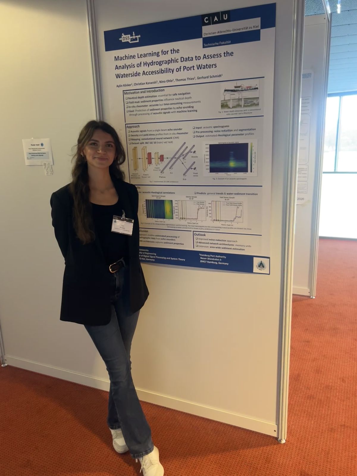 In March 2026, the DSS Chair attended the annual DAGA conference in Dresden. Thanks to the support of the GaS-Club, the student Aylin Kösker was given the opportunity to accompany the chair and participate in the conference from March 23rd to March 26th. As part of the daily poster sessions, she presented the results of her bachelor’s thesis “Machine Learning for the Analysis of Hydrographic Data to Assess the Waterside Accessibility of Port Waters” in the field of Underwater Acoustics. The thesis forms an important basis for an ongoing university research project on the acoustic analysis of sediment properties in harbor areas. The poster session enabled valuable discussions with researchers and conference participants from related research fields.