Lecture "Advanced Digital Signal Processing"
| Basic Information | |
|---|---|
| Lecturers: | Gerhard Schmidt (lecture) and Henning Eikens (exercise) |
| Room: | Building F, room F-SR-II |
| E-mail: | |
| Language: | English |
| Target group: | Students in electrical engineering and computer engineering |
| Prerequisites: | Basic Knowledge about signals and systems |
| Contents: |
Students attending this lecture should be able to implement efficient and robust signal processing structures. Knowledge about moving from the analog to the digital domain and vice versa including the involved effects (and trap doors) should be acquired. Also differences (advantages and disadvantages) between time and frequency domain approaches should be learnt. Topic overview:
|
| References: | J. G. Proakis, D. G. Manolakis: Digital Signal Processing: Principles, Algorithms, and Applications, Prentice Hall, S. K. Mitra: Digital Signal Processing: A Computer-Based Approach, McGraw Hill Higher Education, 2000 A. V. Oppenheim, R. W. Schafer: Discrete-time signal processing, Prentice Hall, 1999, 2nd edition M. H. Hayes: Statistical Signal Processing and Modeling, John Wiley and Sons, 1996 |
News
There will be no lecture or exercise slot on Friday, 7 November 2025, and the slot will be moved to a different date.
Details regarding this will be discussed in the first lecture on Friday 24 October 2025.
There will also be no lecture/exercise slot on Friday 31 October 2025 due to a national holiday.
There will also be no lecture/exercise slot on Friday 08 January 2026 due to the severe weather warning.
Lecture Slides
| Link | Content |
|---|---|
| Slides of the lecture "Introduction" (Contents, literature, analog versus digital signal processing) |
|
| Slides of the lecture "Digital processing of continuous-time signals" (Sampling, Quantization, AD and DA conversion) |
|
| Slides of the lecture "Efficient FIR structures" (DFT and signal processing, FFT, DFT of real sequences) |
|
| Slides of the lecture "DFT/FFT" (DFT and signal processing, FFT, DFT of real sequences) |
|
| Slides of the lecture "Digital filters" (FIR filters, IIR filters, analysis and design) |
|
| Slides of the lecture "Multi-rate digital signal processing" (Upsampling, downsampling, filter banks) |
Exercises
Please note that the questionnaires will be uploaded every week before the excercises, if you download them earlier, you won't get the most recent version.
| Link | Content | Solution |
|---|---|---|
| Exercise 1: Sampling | ||
| Exercise 2: Quantization | ||
| Exercise 3: Discrete Fourier Transform (DFT) / Convolution | ||
| Exercise 4: FFT / Radix-2-FFT | ||
| Exercise 5: FFT / FFTs of Real and Complex Signals | ||
| Exercise 6: Signal Flow Graph | ||
| Exercise 7: Round-off Effects in Digital Filters | ||
| Exercise 8: FIR Filter Design | ||
| Exercise 9: IIR Filter Design | ||
| Exercise 10: Multirate Digital Signal Processing |
Evaluation
The completed evaluations of the last years can be found here. Please note that this page contains the evaluations of all of our lectures. As a consequence you must scroll down to get to the evaluations of this lecture.
Matlab demos
Matlab file for the comparison of window sequences (click to expand)
%**************************************************************************
% Comparison of "standard" and a bit more "advanced" window functions
%**************************************************************************

%**************************************************************************
% Basis parameters
%**************************************************************************
N_win =   64;
N_dft = 1024*16;

%**************************************************************************
% Basic windows - rectangle window
%**************************************************************************
h_rec     = ones(N_win,1);
h_rec     = h_rec / sum(h_rec);

H_rec     = fft(h_rec,N_dft);
H_rec     = H_rec(1:N_dft/2+1);
H_rec_log = 20*log10(abs(H_rec)+eps);

%**************************************************************************
% Basic windows - Hann window
%**************************************************************************
h_han     = hann(N_win);
h_han     = h_han / sum(h_han);

H_han     = fft(h_han,N_dft);
H_han     = H_han(1:N_dft/2+1);
H_han_log = 20*log10(abs(H_han)+eps);

%**************************************************************************
% Basic windows - Hamming window
%**************************************************************************
h_ham     = hamming(N_win);
h_ham     = h_ham / sum(h_ham);

H_ham     = fft(h_ham,N_dft);
H_ham     = H_ham(1:N_dft/2+1);
H_ham_log = 20*log10(abs(H_ham)+eps);

%**************************************************************************
% Advanced windows - "Chebyshev" window
%**************************************************************************
h_che     = chebwin(N_win,10);
h_che     = h_che / sum(h_che);

H_che     = fft(h_che,N_dft);
H_che     = H_che(1:N_dft/2+1);
H_che_log = 20*log10(abs(H_che)+eps);

%**************************************************************************
% Advanced windows - "Prolate" window
%**************************************************************************
h_pro     = dpss(N_win,1.18);
h_pro     = h_pro / sum(h_pro);

H_pro     = fft(h_pro,N_dft);
H_pro     = H_pro(1:N_dft/2+1);
H_pro_log = 20*log10(abs(H_pro)+eps);

%**************************************************************************
% Show results
%**************************************************************************
fig = figure(1);
f = (0:N_dft/2)/N_dft*2;

plot(f,H_rec_log,'b', ...
     f,H_han_log,'r', ...
     f,H_ham_log,'k', ...
     f,H_che_log,'m', ...
     f,H_pro_log,'c', ...
     'LineWidth',2);
legend('Rectangle window', ...
       'Hann window', ...
       'Hamming window', ...
       'Chebyshev window', ...
       'Prolate spheroidal window')
grid on;
xlabel('Normalized frequency \(\Omega/\pi\)','interpreter','latex');
ylabel('dB')
ylim([-90 10])
Matlab file for the effects of quantization on filter design (click to expand)
%**************************************************************************
% Design parameters
%**************************************************************************
N   =  8;     % Filter order
f_c =  0.1;   % Normalized cut-off frequency (0 ... 1)
R_p =  0.5;   % Ripple in dB in passband
R_s = 80;     % Stopband attenuation in dB

%**************************************************************************
% Design of an elliptic lowpass filter
%**************************************************************************
[b,a] = ellip(N, R_p, R_s, f_c);

%**************************************************************************
% Show frequency response
%**************************************************************************
fig = figure(1);
set(fig,'Units','Normalized');
set(fig,'Position',[0.1 0.1 0.8 0.8]);
[H,Omega] = freqz(b,a,2048*4,'whole',2);
plot(Omega,20*log10(abs(H)+eps),'b','LineWidth',2);
grid on
axis([0 2 (-R_s -20) 20])
xlabel('Normalized frequency \Omega/\pi')
ylabel('dB')


%**************************************************************************
% Quantization
%**************************************************************************
B = 32; % Number of bits

a_max = max(abs(a));
b_max = max(abs(b));

a_q = round(a / a_max * 2^B) / 2^B * a_max;
b_q = round(b / b_max * 2^B) / 2^B * b_max;

%**************************************************************************
% Show frequency response of quantized filter
%**************************************************************************
[H_q,Omega] = freqz(b_q,a_q,2048*4,'whole',2);
hold on;
plot(Omega,20*log10(abs(H_q)+eps),'r','LineWidth',2);
hold off;
legend('Non-quantized',['Quantized with ',num2str(B),' bits'])

%**************************************************************************
% Show coefficients
%**************************************************************************
format long;
a
a_q
b
b_q

%**************************************************************************
% Transform to cascade of biquad filters
%**************************************************************************
[sos,g] = tf2sos(b,a);

[L,L_tmp] = size(sos);

sos_q = round(sos / max(max(abs(sos))) * 2^B) / 2^B * max(max(abs(sos)));
g_q   = round(g^(1/L) * 2^B) / 2^B;

H_bq_q = freqz(g_q*sos_q(1,1:3),sos_q(1,4:6),2048*4,'whole',2);
for k = 2:L
    H_bq_q = H_bq_q .* freqz(g_q*sos_q(k,1:3),sos_q(k,4:6),2048*4,'whole',2);
end;

%**************************************************************************
% Show frequency response of quantized biquad filters
%**************************************************************************
[H_q,Omega] = freqz(b_q,a_q,2048*4,'whole',2);
hold on;
plot(Omega,20*log10(abs(H_bq_q)+eps),'k','LineWidth',2);
hold off;
legend('Non-quantized',['Quantized with ',num2str(B),' bits'],...
       'Biquad structure (also qunatized)');
C Examples
C file with different realizations of an FIR filter (click to expand)
#include <math.h>
#include <stdlib.h>
#include <time.h>
#include <stdio.h>

// Parameters (as defines)
#define FILTERLENGTH 1000
#define SIGNALLENGTH 1000000

// Parameters (as variables)
int iRingbufferOffset;

// Vector declarations
float afInput[SIGNALLENGTH];
float afSigBuffer[FILTERLENGTH];
float afCoeffBuffer[FILTERLENGTH];

// Output vector declarations
float afOutput0[SIGNALLENGTH];
float afOutput1[SIGNALLENGTH];
float afOutput2[SIGNALLENGTH];
float afOutput3[SIGNALLENGTH];
float afOutput4[SIGNALLENGTH];

float fLocResult;
float fTmp;

// Time declarations
clock_t tStart, tEnd;
double dTime;

// Counter
int n, m, k;

// Float random number from -1.0 to 1.0
float float_rand()
{
   float max = 1.0;
   float min = -1.0;
   float scale = (float)rand() / (float)RAND_MAX; /* [0, 1.0] */
   return min + scale * (max - min);       /* [min, max] */
}

// Main function
int main()
{
   // Initialize arrays
   for (m = 0; m < FILTERLENGTH; m++)
   {
      afSigBuffer[m] = 0.0;
      afCoeffBuffer[m] = (float)1.0 / (float)(m + 1);
   }
   for (n = 0; n < SIGNALLENGTH; n++)
   {
      afInput[n] = float_rand();
      afOutput0[n] = 0.0;
      afOutput1[n] = 0.0;
      afOutput2[n] = 0.0;
      afOutput3[n] = 0.0;
      afOutput4[n] = 0.0;
   }

   /*-------------------------------------------------------------------------------*
    * Linear buffer with direct memory write
    *-------------------------------------------------------------------------------*/

   // Start timer
   tStart = clock();

   // Clear input buffer
   for (m = 0; m < FILTERLENGTH; m++)
   {
      afSigBuffer[m] = 0.0;
   }

   for (n = 0; n < SIGNALLENGTH; n++)
   {
      // Update linear buffer
      for (m = FILTERLENGTH - 1; m > 0; m--)
      {
         afSigBuffer[m] = afSigBuffer[m - 1];
      }
      afSigBuffer[0] = afInput[n];

      // Calculate filter output
      for (m = 0; m < FILTERLENGTH; m++)
      {
         afOutput0[n] += afSigBuffer[m] * afCoeffBuffer[m];
      }
   }

   // End timer and print time difference
   tEnd = clock();
   dTime = ((double)tEnd - (double)tStart) / (double)CLOCKS_PER_SEC;
   printf("Time for linear buffer with direct memory write is:   %f s\n", dTime);

   /*-------------------------------------------------------------------------------*
    * Linear buffer with local result variable
    *-------------------------------------------------------------------------------*/

   // Start timer
   tStart = clock();

   // Clear input buffer
   for (m = 0; m < FILTERLENGTH; m++)
   {
      afSigBuffer[m] = 0.0;
   }

   for (n = 0; n < SIGNALLENGTH; n++)
   {
      // Update linear buffer
      for (m = FILTERLENGTH - 1; m > 0; m--)
      {
         afSigBuffer[m] = afSigBuffer[m - 1];
      }
      afSigBuffer[0] = afInput[n];

      fLocResult = 0.0;
      // Calculate filter output
      for (m = 0; m < FILTERLENGTH; m++)
      {
         fLocResult += afSigBuffer[m] * afCoeffBuffer[m];
      }
      afOutput1[n] = fLocResult;
   }

   // End timer and print time difference
   tEnd = clock();
   dTime = ((double)tEnd - (double)tStart) / (double)CLOCKS_PER_SEC;
   printf("Time for linear buffer with local result variable is: %f s\n", dTime);

   /*-------------------------------------------------------------------------------*
    * Ringbuffer with if-condition
    *-------------------------------------------------------------------------------*/

   // Start timer
   tStart = clock();

   // Initialize ringbuffer offset
   iRingbufferOffset = FILTERLENGTH - 1;

   // Clear input buffer
   for (m = 0; m < FILTERLENGTH; m++)
   {
      afSigBuffer[m] = 0.0;
   }

   for (n = 0; n < SIGNALLENGTH; n++)
   {
      // Update buffer
      afSigBuffer[iRingbufferOffset] = afInput[n];

      // Calculate filter output
      fLocResult = 0.0;
      for (m = 0, k = iRingbufferOffset; m < FILTERLENGTH; m++)
      {
         fLocResult += afCoeffBuffer[m] * afSigBuffer[k];

         if (++k >= FILTERLENGTH)
         {
            k = 0;
         }
      }
      afOutput2[n] = fLocResult;

      // Update iRingbufferOffset
      if (--iRingbufferOffset < 0)
      {
         iRingbufferOffset = FILTERLENGTH - 1;
      }
   }

   // End timer and print time difference
   tEnd = clock();
   dTime = ((double)tEnd - (double)tStart) / (double)CLOCKS_PER_SEC;
   printf("Time for ringbuffer is:                               %f s\n", dTime);

   /*-------------------------------------------------------------------------------*
    * Ringbuffer with partitioned convolution
    *-------------------------------------------------------------------------------*/

   iRingbufferOffset = FILTERLENGTH - 1;

   // Start timer
   tStart = clock();

   // Clear input buffer
   for (m = 0; m < FILTERLENGTH; m++)
   {
      afSigBuffer[m] = 0.0;
   }

   for (n = 0; n < SIGNALLENGTH; n++)
   {
      // Update ringbuffer
      afSigBuffer[iRingbufferOffset] = afInput[n];

      fLocResult = 0.0;
      // Calculate first part of filter output (0 ... iRingbufferOffset)
      for (m = 0, k = iRingbufferOffset; k < FILTERLENGTH; m++, k++)
      {
         fLocResult += afSigBuffer[k] * afCoeffBuffer[m];
      }

      // Calculate second part of filter output
      for (k = 0; m < FILTERLENGTH; m++, k++)
      {
         fLocResult += afSigBuffer[k] * afCoeffBuffer[m];
      }

      afOutput3[n] = fLocResult;

      // Update iRingbufferOffset
      if (--iRingbufferOffset < 0)
      {
         iRingbufferOffset = FILTERLENGTH - 1;
      }
   }

   // End timer and print time difference
   tEnd = clock();
   dTime = ((double)tEnd - (double)tStart) / (double)CLOCKS_PER_SEC;
   printf("Time for ringbuffer with partitioned convolution is:  %f s\n", dTime);

   /*-------------------------------------------------------------------------------*
    * Ringbuffer with unrolling by hand
    *-------------------------------------------------------------------------------*/

   iRingbufferOffset = FILTERLENGTH - 1;

   // Start timer
   tStart = clock();

   // Clear input buffer
   for (m = 0; m < FILTERLENGTH; m++)
   {
      afSigBuffer[m] = 0.0;
   }

   for (n = 0; n < SIGNALLENGTH; n++)
   {
      // Update ringbuffer
      afSigBuffer[iRingbufferOffset] = afInput[n];

      fLocResult = 0.0;
      // Calculate first part of filter output (0 ... iRingbufferOffset)
      k = iRingbufferOffset;
      m = 0;
      for (; k < FILTERLENGTH - 6; m += 6, k += 6)
      {
         fLocResult += (afSigBuffer[k] * afCoeffBuffer[m] + afSigBuffer[k + 1] * afCoeffBuffer[m + 1] + afSigBuffer[k + 2] * afCoeffBuffer[m + 2] + afSigBuffer[k + 3] * afCoeffBuffer[m + 3] + afSigBuffer[k + 4] * afCoeffBuffer[m + 4] + afSigBuffer[k + 5] * afCoeffBuffer[m + 5]);
      }
      for (; k < FILTERLENGTH; k++, m++)
      {
         fLocResult += afSigBuffer[k] * afCoeffBuffer[m];
      }

      // Calculate second part of filter output
      k = 0;
      for (; m < FILTERLENGTH - 6; m += 6, k += 6)
      {
         fLocResult += (afSigBuffer[k] * afCoeffBuffer[m] + afSigBuffer[k + 1] * afCoeffBuffer[m + 1] + afSigBuffer[k + 2] * afCoeffBuffer[m + 2] + afSigBuffer[k + 3] * afCoeffBuffer[m + 3] + afSigBuffer[k + 4] * afCoeffBuffer[m + 4] + afSigBuffer[k + 5] * afCoeffBuffer[m + 5]);
      }
      for (; m < FILTERLENGTH; k++, m++)
      {
         fLocResult += afSigBuffer[k] * afCoeffBuffer[m];
      }

      afOutput4[n] = fLocResult;

      // Update iRingbufferOffset
      if (--iRingbufferOffset < 0)
      {
         iRingbufferOffset = FILTERLENGTH - 1;
      }
   }

   // End timer and print time difference
   tEnd = clock();
   dTime = ((double)tEnd - (double)tStart) / (double)CLOCKS_PER_SEC;
   printf("Time for ringbuffer unrolling by hand is:             %f s\n", dTime);

   /*-------------------------------------------------------------------------------*
    * Check for errors in convolution (linear buffer as assumed true result)
    *-------------------------------------------------------------------------------*/

   float fConvTest1 = (float)0.0;
   float fConvTest2 = (float)0.0;
   float fConvTest3 = (float)0.0;
   float fConvTest4 = (float)0.0;

   for (n = 0; n < SIGNALLENGTH; n++)
   {
      fConvTest1 += (float)fabs(afOutput0[n] - afOutput1[n]);
      fConvTest2 += (float)fabs(afOutput0[n] - afOutput2[n]);
      fConvTest3 += (float)fabs(afOutput0[n] - afOutput3[n]);
      fConvTest4 += (float)fabs(afOutput0[n] - afOutput4[n]);
   }
   printf("\n");
   printf("Summed absolute error for ringbuffer with direct memory writing is: %f\n", fConvTest1);
   printf("Summed absolute error for ringbuffer is: %f\n", fConvTest2);
   printf("Summed absolute error for ringbuffer with partitioned convolution is: %f\n", fConvTest3);
   printf("Summed absolute error for unrolling by hand is: %f\n", fConvTest4);

   return 0;
}
Exams
Remember to register for the exam in the QiS system! And book a time-slot for your oral exam using this form.
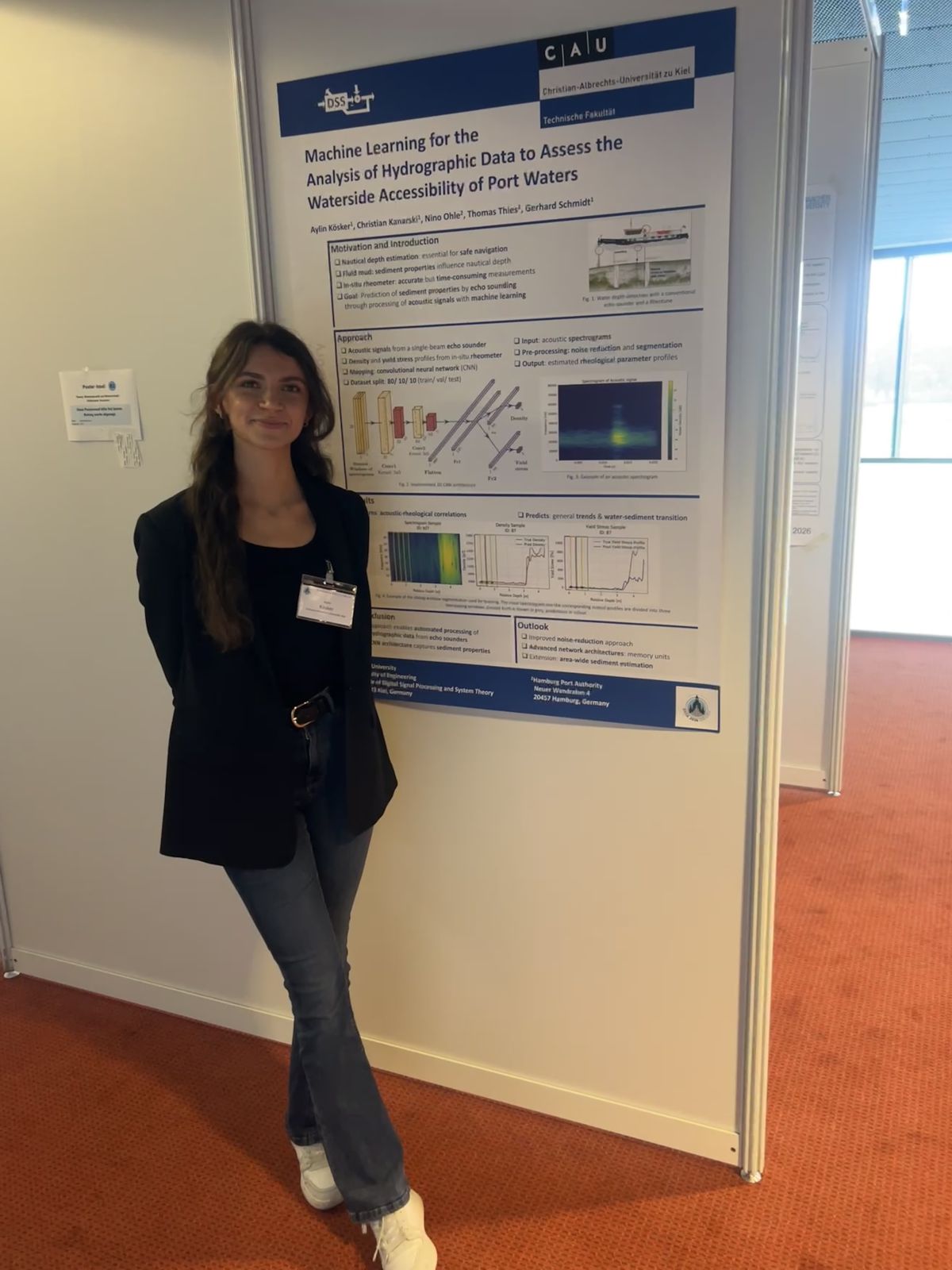 In March 2026, the DSS Chair attended the annual DAGA conference in Dresden. Thanks to the support of the GaS-Club, the student Aylin Kösker was given the opportunity to accompany the chair and participate in the conference from March 23rd to March 26th. As part of the daily poster sessions, she presented the results of her bachelor’s thesis “Machine Learning for the Analysis of Hydrographic Data to Assess the Waterside Accessibility of Port Waters” in the field of Underwater Acoustics. The thesis forms an important basis for an ongoing university research project on the acoustic analysis of sediment properties in harbor areas. The poster session enabled valuable discussions with researchers and conference participants from related research fields.